Confidence Intervals and Hypothesis Testing
520 likes | 791 Vues
Confidence Intervals and Hypothesis Testing. Making Inferences. In this unit we will use what we know about the normal distribution, along with some new information, to make inferences about populations. Before we can do that, we need to understand more about sampling.

Confidence Intervals and Hypothesis Testing
E N D
Presentation Transcript
Making Inferences • In this unit we will use what we know about the normal distribution, along with some new information, to make inferences about populations. • Before we can do that, we need to understand more about sampling.
Sampling Distribution of Means • The sampling distribution of means is what you get when you repeatedly draw a sample and calculate the mean, then plot all of the means. • This distribution has three important properties.
Sampling Distribution of Means Property 1 • The mean of all sample means ( ) is μ. • Say “mu sub X bar.” • If we could draw an infinite number of random samples, the mean of our sample means would be the same as the population mean.
Sampling Distribution of Means Property 2 • The larger the sample size, the closer the sampling distribution of means will be to the normal curve.
Sampling Distribution of Means Property 3 • The larger the size of each sample, the smaller the standard deviation of the sampling distribution of means. • See pp. 172 and 173 in your book.
Standard Error of the Mean • The standard deviation of the sampling distribution of means is called the standard error of the mean. • For the population: • So, if we have the population standard deviation, we can calculate the standard error of the mean.
Estimated Standard Error of the Mean • But we rarely have the population standard deviation, so let’s talk about the sample. • Without population data we can only estimate the standard error of the mean, but the formula is the same:
Why are we computing this? • What did we use the standard deviation for in our last unit? • That’s right, we used it as a unit of measurement to estimate probabilities associated with the normal distribution. • We can use the estimated standard error of the mean to do the same thing, but there are two important differences.
1. The t Distribution • Because our estimates contain error, they do not conform to the normal (z) distribution. • Instead, we will use thetdistribution, a family of distributions. • The t distribution you use will depend on the size of your sample • The larger your sample, the closer thetdistribution gets to the normal distribution.
2. Degrees of Freedom • Because we have a limited sample size, we lose a “degree of freedom.” • All this amounts to (for our purposes), is that we have to again use N-1 when finding our t scores.
Confidence Intervals • When we get a sample mean, we do not know exactly how close it is to the population mean, but we can estimate the probability that the population mean is within a certain range of our obtained sample mean. • The confidence interval is a range of values within which we are reasonably certain the population mean lies.
Confidence Intervals • It is customary to calculate 95% and 99% confidence intervals. • If we find the 95% confidence interval, there is a 5% chance that the population mean falls outside our interval.
Confidence Intervals • Computing the CI involves finding the cutoff scores at the distribution at which we can expect 5% or 1% of the scores to fall. We already know how to do this.
Confidence Intervals • The only problem is that the formula we have for converting our z-score (e.g. 1.96) to a raw score does not work with sample data (remember, we are working with t distributions now). • Luckily, we have a formula that will work:
Confidence Intervals • Don’t be frightened, let’s break it down: This is what we are finding, the confidence interval. Because it is an interval, we will have two values, lower and upper This means we are going to add and subtract what follows from the mean. This is our old friend, the sample mean. This is our estimated standard error of the mean: We are going to learn how to find this value in a table.
Finding t • Go to the “critical values for t” table (table B in Appendix 4). • This is where our N-1 from our lost degree of freedom comes in to play. Under the column labeled df, locate the value of N-1. • Then go over to the value in the 5% column (or the 1% column for your 99% CI).
But What is Happening? • First, compare the t-distribution with a normal distribution. Notice that it is flatter and the tails do not go down near zero so quickly.
But What is Happening? • This means that, by using the t-distribution, we will have to have a larger interval to capture 95% of the area under the curve.
But What is Happening? • The smaller the sample, the larger the interval will be. With a very small sample, the interval will be so large that it will probably be useless.
But What is Happening? • But with larger samples, the t-distribution gets closer to the standard (z) distribution and, therefore, our confidence intervals are smaller and more useful.
But What is Happening? • Second, think of what we are doing as finding the interval where the population mean will fall 95% (or 99%) of the time if we keep taking samples and calculating confidence intervals. We are 95% sure μ is in here somewhere.
But What is Happening? • The beauty of the confidence interval is that it tells you the raw scores for the upper limit and lower limit of the interval, so you can think in terms of raw scores rather than z-scores, which are a bit more abstract. We are 95% sure μ is in here somewhere.
Let’s Try One • Suppose the digit span of 31 adults has been measured, with the result that ΣX = 220.41 and ΣX2 = 1,705.72. What are the 95% and 99% CIs for μ? • Using df = 30 and looking under the 5% and 1% column, we see that t30 is 2.0423 (5%) and 2.75 (1%).
Now We Solve • For our 95% CI: • For our 99% CI:
Activity #1 • As part of its hiring procedure, a large company administers a standardized personality scale to job applicants. Fifty-four applicant for a quality control position have a mean score of 54.2, with s = 16.1, on the dimension of Conscientiousness. • What is the 95% confidence interval for μ? • What is the 99% confidence interval for μ? • If we know that μ for the general population is 49.8, do we have reason to believe that the applicants have a higher level of conscientiousness than the general population?
How Do We Talk About It? • Now that we know how to compute confidence intervals, how do we talk about them? • Template: “We can be 9__% confident that the population mean for _____ is at least [L] and at most [U].”
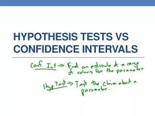
Hypothesis Testing • Because we never know what the next study might show, we can never prove anything. Instead, we focus on disproving things. • We use two types of hypotheses to accomplish this: • The Null Hypothesis (H0) • The Alternative Hypothesis (H1)
The Null Hypothesis H0 • H0 states that your intervention has no effect. • More specifically, it says that your sample is no different from the population. H0: μ = μ0 • If we find no reason to think that there is a difference, we say that we “retain the null.”
The Alternative Hypothesis H1 • H1 states that your intervention does have an effect. • More specifically, it says that there is a difference between your sample and the population. H1: μ ≠ μ0 • If we find good reason to think that there is a difference, we say that we “reject the null.”
Hypothesis Testing • Remember, we can never say that we have proven our treatment to be effective. • If we think we have an effect, we can only say that we reject the null. • This means that we have reason to believe that our sample is different from the population, and our reason is attached to a certain probability (usually 95% or 99%).
One-sample ttest • If we know the population mean and want to know if our sample mean is different, we can conduct a one-sample ttest. • The first step is finding the t score for you sample mean. • The formula for determining the t score should look very familiar:
One-sample t test • It is exactly the same as the formula for determining z-scores, except that we are subtracting the sample mean from the population mean and using the estimated standard error of the mean instead of the standard deviation.
One-sample ttest • When you have your t score, you can use the same t table to determine the probability of obtaining your tscore if your sample mean is the same as the population mean. • Notice the wording in the previous sentence. This is the essence of hypothesis testing. Assuming that the population mean is identical to your sample mean, what is the probability of obtaining the scores that you just obtained?
Alpha Level α • Before you can find out if your sample mean is “significantly” different from your population mean, you have to decide what result will be “significant.” • The “level of significance” is also called the alpha (α) level. The two α levels we have been talking about are α = .05 and α = .01 • The smaller the alpha level, the larger the difference will have to be for your findings to be “significant.”
One-sample t test • If you decided to go with α = .05, you would go to the ttable and find the row associated with your df, then go over to the 5% column. • If your obtained t (tobt)is LARGER than the one listed in the table (tcrit), you have a significant result and can reject the null. The value listed in the table is called the “critical value” (hence tcrit). • If your tobtis SMALLER than tcrit, you retain the null.
Let’s Try It • Trying to encourage people to stop driving to campus, the university claims that on average it takes people 30 minutes to find a parking space on campus. You don’t think it takes so long to find a spot. In fact you have a sample of the last five times you drove to campus, and calculated Xbar = 20. Assuming that the time it takes to find a parking spot is normal, and that s = 6 minutes, then perform a hypothesis test with α level = .05 to see if your claim is correct.
Step 1 • State your hypotheses: • H0: μ = 30. There is no difference between the time it takes you to park and the time the university says it takes to park. (In other words your sample mean is low because of sampling error.) • H1: μ ≠ 30. There is a difference between the time it takes you to park and the time the university says it takes to park.
Step 2 • Make a rejection rule: • Since we already decided to set α = .05, the rule will be to reject the null hypothesis if the absolute value of tobt is greater than tcritin the 5% column. • Here is the rejection rule: Reject H0 if |tobt| ≥ |tcrit .05 • According to the table, tcritis 2.7764 (remember, our dfis 4, and we are looking under 5%).
Step 3 • Find tobt • First we find the estimated standard error of the mean: • Second we find t:
Step 4 • Make the decision. • We know that tcrit = 2.7764 • We know that tobt = -3.727 • So what do we do? • Because the absolute value of tobt is larger than tcrit we reject the null.
Step 5 • Interpret the results: • A one-sample ttest was conducted to test the claim that the mean parking time is 30 minutes The mean parking time obtained from the sample was significantly different from the claimed mean parking time, t(4) = -3.727, p < .05.
p • p is the probability of obtaining a test statistic at least as extreme as the one observed, assuming the null hypothesis is true. • pis the area under the curve beyond positive and negative tobt. • Oftentimes, we will just say whether pis less than or greater than our α level. (e.g., p< .01)
Type I Error (α error) • Hopefully, you have noticed that our decisions are based on probabilities, and improbable things sometimes happen (e.g., people die in plane crashes and get struck by lightning). • One improbable but very possible event is rejecting the null when the null is actually true. If we set α = .05, there is a 5% chance of this happening.
Type I Error (α error) • If there was no difference between our sample and the population and we repeated our study 100 times, we would incorrectly reject the null about 5 times (with α = .05). • One solution is to set α = .01. Even then you will incorrectly reject the null 1% of the time, but that is better than 5%. • But by shrinking your α level, you are increasing the chance of another type of error.
Type II Error (β error) • As you might have guessed, type II error is when you incorrectly retain the null. • In other words, there actually IS a difference, but you did not reject the null. • The higher the requirement for rejecting the null (the smaller the α level), the more likely it is that you will commit a type II error.
Power • Power = 1 - β • β is the probability of committing a type II error, which we cannot know without population parameters. • If we can increase β, we can improve our chances of detecting an effect if there is one.