Chapter 12- Consumption, Real GDP, Multiplier

1. Chapter 12- Consumption, Real GDP, Multiplier

2. Consumption Function I The consumption function is the relationship between consumption (household sector spending) and disposable income. In the consumption function, consumption is directly related to disposable income and is positive even at zero disposable income:

3. The 45-Degree Line The 45-degree line represents all points where consumption and income are exactly equal. C = YD

4. 2000 1999 C = YD 1998 1997 1996 1995 1994 1993 1992 1991 1990 1989 1988 1987 1986 1985 1984 1983 1982 1981 1980 Actual consumer spending 45° U.S. Consumption and Income $7000 6000 5000 CONSUMPTION (billions of dollars per year) 4000 3000 2000 1000 0 $1000 2000 3000 4000 5000 6000 7000 DISPOSABLE INCOME (billions of dollars per year)

5. Autonomous Income Have you ever known people who spend money with out any income? 2. When disposable income is 0 and consumption still exists (food, clothing, shelter- basics) this is autonomous consumption 3. Whether one has to dig into one’s savings, go on welfare, or else beg, borrow or steal, or call mom, one will spend that minimum amount

6. How does this work? Income is low- households tend to Dissave..(borrow from savings or borrow from other sources) Income increases- household aggregate income eventually equals and exceeds current consumption

7. The Keynesian model assumes that there is a positive relationship between consumption and income. Planned ConsumptionExpenditures(trillions of dollars) 45º Line 12 Saving C 9 6 Dis-saving 3 Real Disposable Income(trillions of dollars) 3 6 9 12 45º • However, as income increases, consumption increases by a smaller amount. • Thus, the slope of the consumption function (line C) is less than 1 • (less than the slope of the 45° line).

8. Disposable Income Yd= C+S If we spend… cannot save. If we spend… more activity (production) takes place in the economy… potential to increase GDP What happens if we do not save at all?

9. What is the deciding factor on whether you spend or not? Income Keynes felt we could learn a lot about consumption by focusing on the relationship between income and spending. He said income and consumer spending rise in tandem.. If you know how much income consumers have to spend (Yd), you can predict what they will spend

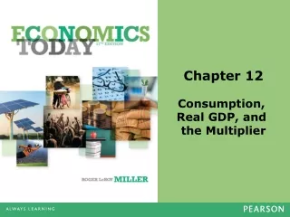
10. Keyne’s Consumption Function Keynes referred to this as “fundamental law” that men are disposed as a rule and on the average, to increase their consumption as their incomeincreases, but not by as much as the increase in their income. *1)At low levels of aggregate income, the consumption expenditures of households will exceed their disposable income (when household income is low, households dissave- they either borrow or draw from past savings to purchase consumption goods

11. E Saving D C Dissaving Consumption Function C = $50 + 0.75YD B G A 45 Degree Line 45 Degree Line C = YD $50 100 150 200 250 300 350 400

12. Keynes Cont. As with most theories, Keynes asks us to assume away a lot of the problem. We will assume there is a specific employment level of output. NARU is present when full-employment capacity is attained. Wages and prices are completely inflexible until full employment is reached Government’s taxing, spending and monetary policies are constant.

13. Keynes said that the economy needs to be directed to full-employment through aggregate expenditures. (C + I + G + X-M )

14. A sluggish economy There are a number of ways to jump-start the economy… Fiscally: taxing & spending. Affects on AD Should the classical or Keynesian approach be used…. Or should an eclectic approach be used?

15. Keynesian Economics • Works only on the AD curve • Assumes AS is stationary • Critics of Keynes: • …But this will cause deficits! • …But the government can’t spend that much!

16. Keynes’ Multiplier Effect • Any new spending (G) becomes new income (Y) to someone. • New income (Y) after taxes (T), called disposable income (Yd), is divided into new spending (C) and new saving (S). • Y = C + S + T • Yd = Y – T = C + S • ΔYd = ΔC + ΔS

17. What do you think Marginal Propensity to Consume means??? You get a “windfall.” How much of those $$ will you spend… (marginally?) How much will you save? (marginally?) • Yd = C + S • ΔYd = ΔC + ΔS • Divide through by ΔYd: • 1 = ΔC/ΔYd + ΔS/ΔYd • Define: • marginal propensity to consume (MPC) MPC = ΔC / ΔYd • marginal propensity to save (MPS) MPS = ΔS / ΔYd • 1 = MPC + MPS, always

18. The Multiplier Effect • In each cycle, part of the new income is set aside as saving (MPS). • So, the next round of income-spending is smaller than the previous round. • As new income grows, it ultimately reaches its maximum. • The power of the multiplier effect is controlled by the size of MPS.

19. The Multiplier Effect • Spending multiplier = 1/MPS

20. What really is the multiplier? The multiplier is based on two concepts already covered: GDP is the nation’s expenditure on all the final goods and services produced during the year at market prices. GDP=C+I+G+(X-M) = Aggregate Demand

21. Summary • Y = C + S + T Y is national income • Yd = Y – T = C + SYd is disposable income • MPC = ΔC / ΔYd • MPS = ΔS / ΔYd • MPC + MPS = 1, always • spending multiplier = 1/MPS • tax multiplier = - (spending multiplier – 1)

22. Obviously if C goes up the entire GDP will go up also. When there is any change in spending- it will have a multiplied effect on GDP *When money is spent by one person, it becomes someone else’s income. When someone spends a dollar, perhaps someone who received that dollar would spend 80 cents and of that 80 cents received by the next person perhaps 64 cents… If we add up all the spending generated by that one dollar, it will add up to four or five or six times that dollar… Hence, the name “multiplier.”

23. The multiplier tells us the extent to which the rate of total spending will change in response to an initial change in the flow of expenditure. Any change in spending (C, I, or G.) will set off a chain reaction, Leading to a multiplied change in GDP. If $1 million investment resulted in $4 million additional income, the multiplier would be 4

24. The Multiplier Process 3. Income reduced by $100 billion 4. Consumption reduced by $75 billion Households 7. Income reduced by $75 billion more 8. Consumption reduced by $56.25 billion more Factor markets Product markets 9. And so on 6. Further cutbacks in employment or wages 5. Sales fall $75 billion Business firms 2. Cutbacks in employment or wages 1. $100 billion in unsold goods appear

25. Marginal Propensity To Consume AdditionalIncome(Dollars) AdditionalConsumption(Dollars) ExpenditureStage Round 1 3/4 Round 2 3/4 Round 3 3/4 Round 4 3/4 Round 5 3/4 Round 6 3/4 Round 7 3/4 Round 8 3/4 Round 9 3/4 Round 10 3/4 3/4 All Others Total 4,000,000 3,000,000 3/4 For simplicity (here) it is assumed that all additions to income are either spent domestically or saved. The Multiplier Principle 1,000,000 750,000 750,000 562,500 562,500 421,875 421,875 316,406 316,406 237,305 237,305 177,979 177,979 133,484 133,484 100,113 100,113 75,085 75,085 56,314 225,253 168,939 • The multiplier concept is fundamentally based upon the proportion of additional income that households choose to spend on consumption: the marginal propensity to consume (here assumed to be 75%  3/4). • Here, a $1,000,000 injection is spent, received as payment, saved and spent, received as payment, saved and spent … etc. … until . . . effectively, $4 million is spent in the economy.