Mapping turbulent combustion by Brian Spalding
500 likes | 689 Vues
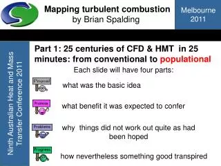
Mapping turbulent combustion by Brian Spalding. Part 1: 25 centuries of CFD & HMT in 25 minutes: from conventional to populational. Each slide will have four parts:. what was the basic idea. what benefit it was expected to confer. why things did not work out quite as had been hoped.

Mapping turbulent combustion by Brian Spalding
E N D
Presentation Transcript
Mapping turbulent combustion by Brian Spalding Part 1: 25 centuries of CFD & HMT in 25 minutes: from conventional to populational Each slide will have four parts: what was the basic idea what benefit it was expected to confer why things did not work out quite as had been hoped how nevertheless something good transpired
THEN I will move the world. No suitable rock. BUT... we have the wheel-barrow, and gear trains and the Archimedean spiral pump which causes swirling flow. Archimedes (267 BC) Give me a lever and a rock to rest it on,
THEN Newton’s laws will determine everything that follows. Too many molecules! BUT... we can predict movements of planets and moons; and of ballistic missiles. Newtonian extrapolators: determinist philosophers Tell us the initial position and velocity of all molecules,
THEN solving our equations will predict all fluid flows. Analytical solution methods were not powerful enough, numerical methods too costly. BUT... simple flows could be analysed, e.g. laminar boundary layers, wakes and jets. Navier and Stokes Suppose we can treat fluids as continua, fully characterised by density and viscosity,
THEN it will do numerical calculations mechanically, i.e. without human labour. It would have needed 25,000 parts, weighed 13,600 kg, been 2.5 m tall. So it was started, but never completed. BUT it paved the thought-way for the electronic digital computer. Charles Babbage I can build a machine consisting of (Archimedean!) gear-wheels and levers;
THEN we will tell you how much surface your equipment needs and how much pumping power. The coefficients could be known only after the equipment had been built. BUT.... James Watt built his separate condenser in 1765 without such knowledge; And so greatly accelerated the Industrial Revolution. Heat-exchanger and furnace designers Give us values of heat- transfer and friction coefficients,
SO design engineers can use our data when expressed in terms of Reynolds, Nusselt and Prandtl numbers. Reynolds Nusselt Prandtl Experiments are expensive; and never numerous enough. Moreover similarity requirements sometimes conflict. BUT correlation-based predictions are better than guesses; so they are used by engineers (with caution). Experimentalists using Similarity Theory Similarity theory predicts full-scale performance from laboratory-scale measurements.
SO we will compute the coefficients and the flow patterns; and experiments will be less needed. Small-scale, rapidly fluctuating eddies (turbulence) govern friction and heat transfer; so the grids required are impossibly fine. BUT... at least laminar flows could now be computed more reliably, swiftly and cheaply than they could be investigated physically. CFD pioneers We have digital computers and Navier-Stokes equations;
Turbulence modellers: Boussinesq, Prandtl, Kolmogorov THEN our equations will calculate effective viscosity ; so turbulent flow can be predicted too. Turbulence entails more than enlarged viscosity; and no model yet predicts correctly the ‘spread angle’ of both plane and round jets. BUT... predictions are often good enough, especially when 'calibrated' using experimental data. Suppose turbulent flows differ from laminar only viaenlargement of effective viscosity,
THEN design and build efficient, cheap, reliable combustors, turbines, etc. Conventional CFD is never 100% reliable, especially for swirling and chemically-reacting flows; BUT... it provides at least some guidance; so CFD software is widely used by engineers. Manufacturers of compressors, turbines, combustion chambers We will employ those ‘good- enough’ methods in (don’t-count-expense) computations; and
THEN surely we shall make better predictions (or so our professors tell us). Computational expense increases greatly, but realism scarcely at all. Why? ‘More-of-the-same’ still omits the essential population-like character of turbulence. BUT closeobservers of turbulent flames could see clearly that a single location is occupied by a population of very different gases at different times. MOTS modellers (MOTS = More Of The Same) If we add more complication to our models, e.g. Reynolds stresses, Large-Eddy Simulation, etcetera,
SO discretising population space as well as distance and time will allow different reaction rates of population elements, to be distinguished. BUT practicability and plausibility of Pop new ideas have been demonstrated, e.g. for chemical-industry reactors. . ‘Populational-CFD’ innovators Treating turbulence as a population-at-each-point phenomenon must enhance realism, !nnovators are far fewer than ‘more-of-the-same’-ers.
How Populational CFD differs from Conventional CFD: 1/9 Both discretise space and time by use of grids of cells, structured or unstructured. Both solve algebraic mass-, momentum - & energy-conservation equations by iterative numerical methods Both take account of (1) sources, (2) diffusion, (3) convection and (4) time-dependence.
How Populational CFD differs from Conventional CFD: 2/9 Here conventional CFD represents 3 neighbouring cells in a structured grid, with 1 temperature for each cell. Populational CFD (next slide) shows the same by discretising temperature, stating how much fluid of each temperature is present. Horizontal position of vertical red lines indicates temperature; with low on the left and high on the right.
How Populational CFD differs from Conventional CFD: 3/9 Here populational CFD represents 3 neighbouring cells in a structured grid with three temperatures for each cell The cell-average temperature is equal to the weighted mean of the three discrete temperatures of the fluid population. PopCFD contains all information of ConCFD and more: viz. distributions. Each cell has some cool, warm and hot fluid in it, but proportions differ. These proportions are measured by the lengths of the brown, green and blue lines.
How Populational CFD differs from Conventional CFD: 4/9 Let time be the independent variable increasing from left to right: as does temperature, So a heat source exists. Populational CFD has come into existence for the reason that:. Conventional CFD cannot simulate turbulent combustion. Chemical-reaction heat sources vary strongly with temperature. So different members of the turbulent population react at different rates. Conventional CFD cannot reflect this.
How Populational CFD differs from Conventional CFD: 5/9 Populational CFD can recognise that: brown fluid is too cold to burn and blue is already burned; but green can burn. To use three temperatures is insufficient; but even as few as three is better than conventional CFD’s one. Populational CFD can simulate turbulent combustion. So brown height stays constant with time, green’s diminishes and blue's grows by the same amount.
How Populational CFD differs from Conventional CFD: 6/9 Conventional CFD accounts for four processes, (sources, diffusion, convection & time-dependence); but Populational CFD accounts for two more: (5) Merging, by way of collision, coupling-and-splitting or engulfment, which influence turbulent combustion,and (6) differential (i.e. selective) convection, which influences buoyant and swirling flows. The next slide explains item (6).
How Populational CFD differs from Conventional CFD: 7/9 Differential convection in vertical direction. 2 members (green & blue) with differing body forces: buoyancy; or centrifugal force in swirling flow. Even a two-member population can explain the well-documented (but woefully ignored) body-force-induced un-mixing process. higher This is encountered in buoyant and swirling flows. lower Early time Late time As time proceeds green fluid moves down and blue fluid up. • The discretized variable could be: • temperature in buoyancy-driven flow • or • circumferential velocity in swirling flow.
How Populational CFD differs from Conventional CFD: 8/9 Those populations (of temperature andcircumferentialvelocity) were one-dimensional.But one may choose to discretise two (or more) variables. Example1. For combustion: 10 temperature and 10 fuel/air ratio intervals in each x~y~z~t cell. The sizes of squares in each population-grid cell show the proportions of time the fluid is in each state.
How Populational CFD differs from Conventional CFD: 9/9 Example 2. For swirling flow, one might choose to discretise the circumferential and radialvelocity components. The population distribution might look like this. Centrifugal force causes high radial velocities. But this is a guess; for no-one has yet done the calculations! Who will be the first to do so?
THEN hoped to distribute the three parts of his kingdom, and enjoy a peaceful old age. His daughters made the play truly into a tragedy. BUT.... maps are used with success by 2D-population modellers of combustion and might be by swirl-flow modellers also. Turbulence cartographers "Give me the map there", commanded King Lear (act 1, scene 1);
THEN populational CFD can solve equations which, for each location, compute population-member-concentration changes resulting from merging and differential convection. Well-tested formulations for differential convection are still lacking; BUT... one can always guess; The turbulent-combustion map-users The population of turbulent reacting gases at a space-time location can be described by contours on a temperature-rise versus fuel-air ratio map. or neglect!
THEN equations for particle movement through this 'population space', based on momentum conservation, could be solved, Differential convection is of the essence; and the 'engulfment' process of population-member -merging must probably be replaced by another. BUT... the turbulent-combustion pattern could be used as a start. A turbulent-swirling-flow map For swirling flows, circumferential velocity and radial velocity are plausible mapco-ordinates.
End of Part 1 Beginning of Part 2 Here ends the 25-century revew Now follows a closer look at turbulent-combustion models from the populational view-point Contents 2.1 Describing further the Tri-Mix ‘map’ of turbulent combustion.. 2.2. Placing models of turbulent combustion on the map. 2.3 Explaining how gas-state distributions can be computed viafinite-volume equations
2.1 The Tri-Mix map;Well-known precursor plots. The right–hand plot shows how the temperature of a fuel-air mixture varies with fuel proportion, when fuel is (upper) fully burned and (lower) fully un-burned. The ‘adiabatic temperature rise’ is the vertical distance between them. The left-hand plot shows the free-fuel and free-oxygen values for the fully-burned condition,. The mixture fraction at which both oxygen and fuel are zero is called ‘stoichiometric’. The ‘TriMix’ diagram is a way of mapping the states which lie between the fully-burned and fully-unburned extremes.
The Tri-Mix map;uses, and nature • The diagram con be used: • for describing fuel+air flames; and • for representing and comparing • theoretical models of combustion. Its horizontal dimension is mass fraction of fuel-derived material, or, in atomic_nitrogen terms: 1.0 - atomic_nitrogen fraction/0.768. Its vertical dimension is the adiabatic temperature rise resulting from complete combustion of the fuel (to CO2 and H20). Points lying outside the triangle correspond to non-physical negative concentrations.
The Tri-Mix map; contours of various thermo-physical attributes If we assume that diffusivities of all gases are equal, C and H oxidise in proportion, and concentrations of O, OH, NO, etc small, then: here are the distributions of unburned fuel (left) and free oxygen (right). Red is high, blue low, in all cases. Here is the (adiabatic) gas temperature (right); and the reactedness (left); Any other properties such as density and viscosity can also be computed and displayed. and finally the concentration of combustionproducts (right).
The Tri-Mix map; contours of various chemical reaction rates Knowing the composition and the temperature, chemical kineticists can (in principle) compute the instantaneous rates of chemical reaction per unit mass of mixture in the various states. There are three kinds of reaction to be considered, of which the rate-contours are shown below (red is high rate; blue is low rate): • the main energy-producing oxidation of the fuel, which is what we desire to promote; 2. the undesired reaction producing oxides of nitrogen; and 3. the often equally-undesired smoke-creating reaction. 4.. Note that we have not yet consideried any particular flame We have simply assembled knowledge about the attributes of all possible members of the gases-in-flame population.
The Tri-Mix map; contours of population-member density products (hot) This contour diagram does relate to a particular flame; and to a particular geometric location. It describes the proportions of time in which the gas at that point is in each of the possible states represented on the state-map. Time proportion means probability or mass fraction or population density. Multiplication by their reaction rates & integration over the triangle gives total rates of heat, NOX & smoke formation. fuel air (cold) The task of simulation of turbulent combustion is therefore ‘simply’ that of determining what this population-density distribution actually is. Of course, this must be done for every location in space; and, for non-steady flames, for each (not too small) instant of time; or rather, for each ‘cell’ in the space-time grid of the computation.
2.2 Putting models on the map; two one-member populations • Modeling means ‘neglecting awkward facts’ such as: • diffusion coefficients do differ somewhat from gas to gas; and • oxidation of the C and H in a hydrocarbon do not proceed at always-proportionate rates. • These neglects are not too far from the truth.. Very far is the often-used NOFMIB model (i.e. NO-Fluctuations, Mixed-Is-Burned). Its ‘population’ is a single point on the upper boundary of the triangle. The horizontal position is determined by solving a single finite-volume equation for the mixturefraction. Little less extreme is NOFL (i.e.NO-FLuctuations), which also uses single-point representation, but does allow the point to be anywhere in the triangle. Two finite-volume equations determine its location: for mixture fraction and for unburned-fuel fraction.
Models on the map:two-member populations The eddy-break-up model(1971) postulated a population of two members, both having the same fuel ratio, but one fully burned & the other fully unburned. The two members were supposed to collide, at rates fixed by hydrodynamic turbulence, forming intermediate-temperature and -composition material which quickly became fully burned. This model provided a (negative) source term in the finite-volume equation for the unburned fuel fraction, often expressed as: - constant * density * r * (1 – r) * e / k where r is the local reactedness of the mixture, so that r : (1-r) is the ratio of burned to unburned material; e &k are from k-epsilon model. This link between hydrodynamics and reaction rate appears in some form, in almost all subsequent models of combustion.
Models on the map the 2-member presumed-pdf model Also in 1971 appeared the first ‘presumed-pdf’ model, which is represented by the two red blobs on the base. (because at first the fluids were non-burning), and by two more on the sides when extended to mixed-is-burned models of turbulent flames. Their locations were computed from two finite-volume equations: for the mixture fraction and for the root-mean-square fluctuations. The second of these (the ‘g-equation’) was novel. The presumed shape of the pdf (i.e. probability-density function) is shown on the left. Variants of this model are still often used.
Another 2-member model on the map two-Navier-Stokes-equations model Invented so as to simulate two-phase (e.g. steam-water) flows, the IPSA algorithm was applied in 1982 to a two-member population of burning gases. It solves mass, momentum and energy equations for both members; predicts their relative motion. In flames propagating in ducts, hotter members (right) overtake colder ones (left); so mixing and combustion are intensified. [Time is UP; distance RIGHT] This model can accommodate and generalise EBU, EDC (see later slide) and presumed–pdf assumptions. But it is seldom used. Why not? Few professors have paid attenion to two-phase-flow CFD. A pity; for this model can do what conventional turbulence models cannot: namely simulate un-mixing.
Models on the map: A four-member-population model Two facts about turbulent pre-mixed flames in plane-walled ducts 1. Increasing flow velocity increases flame speed; flame angle is constant 2. Sufficient increase of velocity extinguishes the flame EBU (2-fluid) explained 1, not 2. The solution (24 years later !) refine the ‘population grid’. Eddy-break-up used a two-member population; so why not try using four? It worked! The presence of the ‘hot, can burn’ fluid (see left) allows space for chemical kinetics. So extinction could be predicted (in principle).
How the four-fluid model allowed for finite chemical reaction rates The Eddy-Break-Up postulate was that fully-burned and fully-unburned gas fragments collided and merged, at concentration-proportional rates, and the resulting mixture combusted instantly. With 4 fluids, there are more pairings possible. Collisions between fluids 1 and 3 created fluid 2, 2 and 4 created fluid 3, 1 and 4 created fluid 2 and also fluid 3. Reaction of fluid 3 created fluid 4 at a chemistry- controlled rate.. Fluids: 1 2 3 4
Applications of the four-fluid modelto transient pre-mixed flames The four-fluid model was used successfully for simulating flame spread in a baffled duct and for oil-platform explosion simulation.
Models on the map: from 4 to many; the multi-fluid model In conventional CFD, we divide space-time into as many intervals as accuracy requires. Why not do the same for the population-defining variable at each point? This worked too! On the left is the calculated pdf of a 40-member population in a ‘well-stirred reactor’. Its shape depends in the relative rates of merging and reaction and on the postulated dependence of the latter on reactedness.. The (truncated) spikes at left and explain the success of the EBU spikes-only presumption.
Models on the map :A fourteen-member 2D population EBU is often applied to non-premixed flames, with dubious validity. So a 1996 fourteen-fluid model was the partly-pre-mixed Bunsen-burner flame. Its TriMix representation is shown on the right. On the left are concentration contours of two of the fluids for a turbulent Bunsen burner. On the right is a 2D probability density function for one point in the flame. (Trimix had not yet been invented).
Other models on the map: 1. eddy-dissipation concept ; 2. flamelet 1. The 1981 EDC postulates a two-member population; its members are (1) the so-called ‘fine structures’, occupying little space; and (2) the remainder; both are shown as blue blobs on the right. It is claimed that the fine-structures location allows the reaction rate of the mixture to be calculated. What a clever blob! 2. The 1980 Flamelet model postulates a population distributed along a vertiical line, from unburned to burned, but (like EBU) with most fluid at the ends. The shape of the distribution is supposed to be the same as in a steadily-propagating laminar pre-mixed flame. But why should it be? The last assumption allowed complex chemical kinetics to be introduced, and much computer time to be consumed. But their dubious basis renders their results correspondingly doubtful.
Other models on the map: 3. ESCIMO (=Engulfment, Stretching, Coherence,Inter-diffusion , Moving Observer) ObserverObserver. The 1976 ESCIMO model also saw small laminar flames as players in turbulent combustion, namely as (more plausible?) rolling-up vortices. These were subjected to one-dimensional unsteady analysis with results as indicated. In contrast to ‘’flamelets’, the ‘engulfed’ and ‘engulfing’ parents of a ‘fold’ could have anytemperature and composition. Therefore an ‘ESCIMO event’ might have been represented on the TriMix diagram by way of a patch as shown on the right. ESCIMO was ‘in advance of its time’; but its ideas may yet come to fruition as part of populational CFD.
Other models on the map:4. the ‘Pdf-Transport’ Model Populations can be completely described in terms of probability-density functions; so the 1981 ‘pdf-transport model’ appeared to meet the need. Unfortunately, its first introducer chose the Monte Carlo method for solving the transport equations, expressed on Tri-Mix as random points. This is legitimate, just as one can computep by counting how many uniformly sprinkled sand particles lie inside and how many outside the circle. But there are quicker ways! Therefore large computing times, and foreign-to-CFD-specialist language, have delayed development of the model. Why is Monte Carlo still used? Look left.
2.3 How population distributions can be best computed Currently fashionable models of combustion (EBU, EDC, flamelet) and turbulence (RANS, LES) lack essential populational ingredients. Pdf-transport is weighed down by its Monte Carlo baggage and unlike-CFD jargon. But discretized-population CFD is as easy to use as conventional CFD; it just has a few extraitems namely: • extra variables, viz mass fractions of each population element; • extra terms in equations , viz. merging; differential convection • extra empirical constants , e.g. for merging_rate / (e/k) • extra research opportunities , e.g. unstructuredpopulation grids • extra avenues to explore , e.g. population-gridrefinement • extra experimentally-testable items, e.g. population-memberconcentrations and attributes
Alexander Pope wrote: ”Be not the first by which the new are tried.” Don’t worry. You won’t be the first. Here is a 30-year old calculation of temperature contours in (one sector of) an idealised gas-turbine combustor, Populational CFD is not all that new. NOFL was the model used
Smoke formation rate is influenced by turbulent fluctuations 20 years later, this combustor was used to show how fluctuations of fuel-air ratio affect predictions of rates of smoke formation. The small differences are significant when CFD is being used to optimise the design. With fluctuations A 10-fluid model was used with fuel-air-ratio as the population-dimension Each cell had its own pdf. Without fluctuations
Computing population distributions; a grid-refinement study 2-, 4-, 14-, 40-, 100- and multi-member populations appear above. But how many does one truly need? There is no general answer. In conventional CFD, the needed sizes of space interval or time step are found bycomparing results obtained with various sizes . The same is true of Populational CFD. Grid-refinement studies must be made, as shown here for a 2D population: Four pdfs for the same geometric location with population grids: 3*3 5*5 7*7 11*11 The Monte-Carlo approach lacks this grid-refinement capability.
Computing population distributions via discretization of TriMix The TriMix plane can be discretised in various ways. The 2D pdf’s just seen used lines of constant Temperature rise and constant Mixture fraction; but that left some cells empty. The grid shown on the left is better, using constant reactedness lines as the second co-ordinate. Finite-volume equations are solved for the mass fraction of gas in each cell. As well as convection and diffusion, these contain terms for reaction and for engulfment. The engulfment-rate formula can be that of EBU, until a better one is discovered.
Computing population distributions via TriMix, for all space locations For each cell in the3D geometric grid covering the combustor (shown 2D here), there corresponds one set of cells in the 2D population grid. So the problem might be thought of as five-dimensional. That term is too alarmist; all that has happened is that the 3D problem has acquired some additionaldependent variables, equal in number to the cells in one 2D population grid, typically between 10 and 100. Thus, without the population dimension, the dependent variables might have been p, u, v, w, ke, eps, f, T; and with it they become been p, u, v, w, ke, eps, f1, f2, f3, ...... f20, say, without immense computer-time increase.
Concluding remarks,1 Populational CFD is ready for application to practical problems. The prospects of realistic combustor modelling via the populational approach are good. But they have been good for fifteen years! Yet resources are still being wasted on too-narrowly-conceived LES, EDC and flamelet models. Why? Too many MOTSmen (MOTS=More Of The Same) Not enough POTSmen (POTS=POpulaTion Student I hope to have shifted the balance today. If only it were as easy as that!
Setbacks are also certain, and (hard-to- find) resourcefulness will be needed. BUT… history shows that old ideas always are replaced by new ones. Concluding remarks, 2 the future IF it is at last recognised that ‘More-Of-The-Same’ turbulence modelling is hopeless, THEN, switching attention to populational modelling will make improved predictive capability certain. So this slide marks only of this lecture, not of continued progress, the END.