Download
1 / 46
590 likes | 1.78k Vues
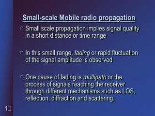
Mobile Radio Propagation - Small-Scale Fading and Multipath. CS 515 Mobile and Wireless Networking Fall 2002 İ brahim K ö rpe oğ lu Computer Engineering Department Bilkent University. Relationship between Bandwidth and Receiver Power.

E N D
Mobile Radio Propagation - Small-Scale Fading and Multipath CS 515 Mobile and Wireless Networking Fall 2002 İbrahim Körpeoğlu Computer Engineering Department Bilkent University
Relationship between Bandwidth and Receiver Power • What happens when two different signals with different bandwidths are sent through the channel? • What is the receiver power characteristics for both signals? • We mean the bandwith of the baseband signal • The bandwidth of the baseband is signal is inversely related with its symbol rate. One symbol ©İbrahim Körpeoğlu
Bandwidth of Baseband Signals Highbandwidth (Wideband) Signal Lowbandwidth (Narrowband) Signal Continuous Wave (CW) Signal t ©İbrahim Körpeoğlu
A pulsed probing signal (wideband) Tbb Transmitter p(t) x(t): transmitted signal TREP Multipath Wireless Channel Multipath Wireless Channel x(t) p(t) y(t) r(t) Baseband signals Bandpass signals ©İbrahim Körpeoğlu
Received Power of Wideband Sİgnals Multipath Wireless Channel p(t) r(t) The output r(t) will approximate the channel impulse response since p(t) approximates unit impulses. Assume the multipath components have random amplitudes and phases at time t. ©İbrahim Körpeoğlu
Received Power of Wideband Sİgnals This shows that if all the multipath components of a transmitted signal is resolved at the receiver then: The average small scale received power is simply the sum of received powers in each multipath component. In practice, the amplitudes of individual multipath components do not fluctuate widely in a local area (for distance in the order of wavelength or fraction of wavelength). This means the average received power of a wideband signal do not fluctuate significantly when the receiver is moving in a local area. ©İbrahim Körpeoğlu
Received Power of Narrowband Sİgnals Transmitter x(t): transmitted signal A CW Signal c(t) Assume now A CW signal transmitted into the same channel. Let comlex envelope will be: The instantaneous complex envelope of the received signal will be: The instantaneous power will be: ©İbrahim Körpeoğlu
Received Power of Narrowband Sİgnals Over a local area (over small distance – wavelengths), the amplitude a multipath component may not change signicantly, but the phase may change a lot.For example: - if receiver moves l meters then phase change is 2p. In this case the component may add up posively to the total sum S. - if receiver moves l/4 meters then phase change is p/2 (90 degrees) . In this case the component may add up negatively to the total sum S, hence the instantaneous receiver power. Therefore for a CW (continues wave, narrowband) signal, the small movements may cause large fluctuations on the instantenous receiver power, which typifies small scale fading for CW signals. ©İbrahim Körpeoğlu
Wideband versus Narrowband Baseband Signals However, the average received power for a CW signal over a local area is equivalent to the average received power for a wideband signal on the local area. This occurs because the phases of multipath components at different locations over the small-scale region are independently distributed (IID uniform) over [0,2p]. In summary: • Received power for CW signals undergoes rapid fades over small distances • Received power for wideband signals changes very little of small distances. • However, the local area average of both signals are nearly identical. ©İbrahim Körpeoğlu
Small-Scale Multipath Measurements • Several Methods • Direct RF Pulse System • Spread Spectrum Sliding Correlator Channel Sounding • Frequency Domain Channel Sounding • These techniques are also called channel sounding techniques ©İbrahim Körpeoğlu
Direct RF Pulse System Tx fc Pulse Generator RF Link Rx Digital Oscilloscope BPF Detector ©İbrahim Körpeoğlu
Parameters of Mobile Multipath Channels • Time Dispersion Parameters • Grossly quantifies the multipath channel • Determined from Power Delay Profile • Parameters include • Mean Access Delay • RMS Delay Spread • Excess Delay Spread (X dB) • Coherence Bandwidth • Doppler Spread and Coherence Time ©İbrahim Körpeoğlu
Measuring PDPs • Power Delay Profiles • Are measured by channel sounding techniques • Plots of relative received power as a function of excess delay • They are found by averaging intantenous power delay measurements over a local area • Local area: no greater than 6m outdoor • Local area: no greater than 2m indoor • Samples taken at l/4 meters approximately • For 450MHz – 6 GHz frequency range. ©İbrahim Körpeoğlu
Timer Dispersion Parameters Determined from a power delay profile. Mean excess delay( ): Rms delay spread (st): ©İbrahim Körpeoğlu
Timer Dispersion Parameters Maximum Excess Delay (X dB): Defined as the time delay value after which the multipath energy falls to X dB below the maximum multipath energy (not necesarily belonging to the first arriving component). It is also called excess delay spread. ©İbrahim Körpeoğlu
RMS Delay Spread ©İbrahim Körpeoğlu
PDP Outdoor ©İbrahim Körpeoğlu
PDP Indoor ©İbrahim Körpeoğlu
Noise Threshold • The values of time dispersion parameters also depend on the noise threshold (the level of power below which the signal is considered as noise). • If noise threshold is set too low, then the noise will be processed as multipath and thus causing the parameters to be higher. ©İbrahim Körpeoğlu
Coherence Bandwidth (BC) • Range of frequencies over which the channel can be considered flat (i.e. channel passes all spectral components with equal gain and linear phase). • It is a definition that depends on RMS Delay Spread. • Two sinusoids with frequency separation greater than Bc are affected quite differently by the channel. f1 Receiver f2 Multipath Channel Frequency Separation: |f1-f2| ©İbrahim Körpeoğlu
Coherence Bandwidth Frequency correlation between two sinusoids: 0 <= Cr1, r2 <= 1. If we define Coherence Bandwidth (BC) as the range of frequencies over which the frequency correlation is above 0.9, then s is rms delay spread. If we define Coherence Bandwidth as the range of frequencies over which the frequency correlation is above 0.5, then This is called 50% coherence bandwidth. ©İbrahim Körpeoğlu
Coherence Bandwidth • Example: • For a multipath channel, s is given as 1.37ms. • The 50% coherence bandwidth is given as: 1/5s = 146kHz. • This means that, for a good transmission from a transmitter to a receiver, the range of transmission frequency (channel bandwidth) should not exceed 146kHz, so that all frequencies in this band experience the same channel characteristics. • Equalizers are needed in order to use transmission frequencies that are separated larger than this value. • This coherence bandwidth is enough for an AMPS channel (30kHz band needed for a channel), but is not enough for a GSM channel (200kHz needed per channel). ©İbrahim Körpeoğlu
Coherence Time • Delay spread and Coherence bandwidth describe the time dispersive nature of the channel in a local area. • They don’t offer information about the time varying nature of the channel caused by relative motion of transmitter and receiver. • Doppler Spread and Coherence time are parameters which describe the time varying nature of the channel in a small-scale region. ©İbrahim Körpeoğlu
Doppler Spread • Measure of spectral broadening caused by motion • We know how to compute Doppler shift: fd • Doppler spread, BD, is defined as the maximum Doppler shift: fm = v/l • If the baseband signal bandwidth is much greater than BD then effect of Doppler spread is negligible at the receiver. ©İbrahim Körpeoğlu
Coherence Time Coherence time is the time duration over which the channel impulse response is essentially invariant. If the symbol period of the baseband signal (reciprocal of the baseband signal bandwidth) is greater the coherence time, than the signal will distort, since channel will change during the transmission of the signal . TS Coherence time (TC) is defined as: TC f2 f1 Dt=t2 - t1 t1 t2 ©İbrahim Körpeoğlu
Coherence Time Coherence time is also defined as: Coherence time definition implies that two signals arriving with a time separation greater than TC are affected differently by the channel. ©İbrahim Körpeoğlu
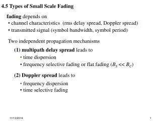
Types of Small-scale Fading ©İbrahim Körpeoğlu
Flat Fading • Occurs when the amplitude of the receivedsignal changes with time • For example according to Rayleigh Distribution • Occurs when symbol period of the transmitted signal is much larger than the Delay Spread of the channel • Bandwidth of the applied signal is narrow. • May cause deep fades. • Increase the transmit power to combat this situation. ©İbrahim Körpeoğlu
Flat Fading h(t,t) r(t) s(t) t << TS 0 t TS+t TS 0 0 Occurs when: BS << BC and TS >> st BC: Coherence bandwidthBS: Signal bandwidth TS: Symbol periodst: Delay Spread ©İbrahim Körpeoğlu
Frequency Selective Fading • Occurs when channel multipath delay spread is greater than the symbol period. • Symbols face time dispersion • Channel induces Intersymbol Interference (ISI) • Bandwidth of the signal s(t) is wider than the channel impulse response. ©İbrahim Körpeoğlu
Frequency Selective Fading h(t,t) r(t) s(t) t >>TS TS 0 TS+t t TS 0 0 Causes distortion of the received baseband signal Causes Inter-Symbol Interference (ISI) Occurs when: BS> BC and TS<st TS<st As a rule of thumb: ©İbrahim Körpeoğlu
Fast Fading • Due to Doppler Spread • Rate of change of thechannel characteristics is larger than theRate of change of thetransmitted signal • The channel changes during a symbol period. • The channel changes because of receiver motion. • Coherence time of the channel is smaller than the symbol period of the transmitter signal Occurs when: BS < BD and TS>TC BS: Bandwidth of the signalBD: Doppler Spread TS: Symbol PeriodTC: Coherence Bandwidth ©İbrahim Körpeoğlu
Slow Fading • Due to Doppler Spread • Rate of change of thechannel characteristics is much smaller than theRate of change of thetransmitted signal Occurs when: BS >> BD and TS<< TC BS: Bandwidth of the signalBD: Doppler Spread TS: Symbol PeriodTC: Coherence Bandwidth ©İbrahim Körpeoğlu
Different Types of Fading TS Flat Fast Fading Flat Slow Fading Symbol Period of Transmitting Signal st Frequency Selective Fast Fading Frequency Selective Slow Fading TC TS Transmitted Symbol Period With Respect To SYMBOL PERIOD ©İbrahim Körpeoğlu
Different Types of Fading BS Frequency Selective Fast Fading Frequency Selective Slow Fading Transmitted Baseband Signal Bandwidth BC Flat Fast Fading Flat Slow Fading BD BS Transmitted Baseband Signal Bandwidth With Respect To BASEBAND SIGNAL BANDWIDTH ©İbrahim Körpeoğlu
Fading Distributions • Describes how the received signal amplitude changes with time. • Remember that the received signal is combination of multiple signals arriving from different directions, phases and amplitudes. • With the received signal we mean the baseband signal, namely the envelope of the received signal (i.e. r(t)). • Its is a statistical characterization of the multipath fading. • Two distributions • Rayleigh Fading • Ricean Fading ©İbrahim Körpeoğlu
Rayleigh and Ricean Distributions • Describes the received signal envelope distribution for channels, where all the components are non-LOS: • i.e. there is no line-of–sight (LOS) component. • Describes the received signal envelope distribution for channels where one of the multipath components is LOS component. • i.e. there is one LOS component. ©İbrahim Körpeoğlu
Rayleigh Fading ©İbrahim Körpeoğlu
Rayleigh Rayleigh distribution has the probability density function (PDF) given by: s2 is the time average power of the received signal before envelope detection. s is the rms value of the received voltage signal before envelope detection Remember: (see end of slides 5) ©İbrahim Körpeoğlu
Rayleigh The probability that the envelope of the received signal does not exceed a specified value of R is given by the CDF: ©İbrahim Körpeoğlu
Rayleigh PDF 0.6065/s mean = 1.2533s median = 1.177s variance = 0.4292s2 5s s 2s 3s 4s ©İbrahim Körpeoğlu
Ricean Distribution • When there is a stationary (non-fading) LOS signal present, then the envelope distribution is Ricean. • The Ricean distribution degenerates to Rayleigh when the dominant component fades away. ©İbrahim Körpeoğlu
Level Crossing Rate (LCR) Threshold (R) LCR is defined as the expected rate at which the Rayleigh fading envelope, normalized to the local rms signal level, crosses a specified threshold level R in a positive going direction. It is given by: ©İbrahim Körpeoğlu
Average Fade Duration Defined as the average period of time for which the received signal is below a specified level R. For Rayleigh distributed fading signal, it is given by: ©İbrahim Körpeoğlu
Fading Model – Gilbert-Elliot Model Fade Period Signal Amplitude Threshold Time t Bad (Fade) Good (Non-fade) ©İbrahim Körpeoğlu
Gilbert-Elliot Model 1/AFD Bad (Fade) Good (Non-fade) 1/ANFD The channel is modeled as a Two-State Markov Chain. Each state duration is memory-less and exponentially distributed. The rate going from Good to Bad state is: 1/AFD (AFD: Avg Fade Duration) The rate going from Bad to Good state is: 1/ANFD (ANFD: Avg Non-Fade Duration) ©İbrahim Körpeoğlu