Part 2: part-based models
Part 2: part-based models. by Rob Fergus (MIT). Problem with bag-of-words. All have equal probability for bag-of-words methods Location information is important. Overview of section. Representation Computational complexity Design choices Recognition Demos Learning Automated methods.

Part 2: part-based models
E N D
Presentation Transcript
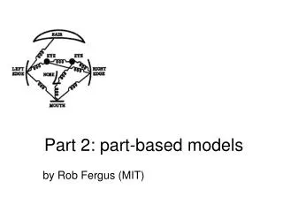
Part 2: part-based models by Rob Fergus (MIT)
Problem with bag-of-words • All have equal probability for bag-of-words methods • Location information is important
Overview of section • Representation • Computational complexity • Design choices • Recognition • Demos • Learning • Automated methods
Representation • Object as set of parts • Generative representation • Model: • Relative locations between parts • Appearance of part • Issues: • How to model location • How to represent appearance • Sparse or dense (pixels or regions) • How to handle occlusion/clutter Figure from [Fischler73]
Example scheme • Model shape using Gaussian distribution on location between parts • Model appearance as pixel templates • Represent image as collection of regions • Extracted by template matching: normalized-cross correlation • Manually trained model • Click on training images
Sparse representation + Computationally tractable (105 pixels 101 -- 102 parts) + Generative representation of class + Avoid modeling global variability + Success in specific object recognition - Throw away most image information - Parts need to be distinctive to separate from other classes
History of Idea • Fischler & Elschlager 1973 • Yuille ‘91 • Brunelli & Poggio ‘93 • Lades, v.d. Malsburg et al. ‘93 • Cootes, Lanitis, Taylor et al. ‘95 • Amit & Geman ‘95, ‘99 • Perona et al. ‘95, ‘96, ’98, ’00 • Felzenszwalb & Huttenlocher ’00 • Many papers since 2000
The correspondence problem • Model with P parts • Image with N possible locations for each part • NP combinations!!!
Connectivity of parts • Complexity is given by size of maximal clique in graph • Consider a 3 part model • Each part has set of N possible locations in image • Location of parts 2 & 3 is independent, given location of L • Each part has an appearance term, independent between parts. Shape Model Factor graph Variables L 2 3 L 2 3 Factors S(L) S(L,2) S(L,3) A(L) A(2) A(3) Shape Appearance
Connectivity of parts • To find best match in image, we want most probable state of L, • Run max-product message passing L 2 3 md ma mb mc S(L) S(L,2) S(L,3) A(L) A(2) A(3) Take O(N2) to compute: For each of the N values of L, need to find max over N states
Different graph structures 6 1 3 5 2 3 2 3 1 2 1 4 5 4 6 4 5 6 Fully connected Star structure Tree structure O(N6) O(N2) O(N2) • Sparser graphs cannot capture all interactions between parts
Some class-specific graphs • Articulated motion • People • Animals • Special parameterisations • Limb angles Images from [Kumar05, Felzenszwalb05]
Regions or pixels • # Regions << # Pixels • Regions increase tractability but lose information • Generally use regions: • Local maxima of interest operators • Can give scale/orientation invariance Figures from [Kadir04]
Hierarchical representations • Pixels Pixel groupings Parts Object • Multi-scale approach increases number of low-level features • [Amit98] • [Bouchard05] Images from [Amit98,Bouchard05]
Translation Translation and Scaling Similarity transformation Affine transformation How to model location? • Explicit: Probability density functions • Implicit: Voting scheme • Invariance • Translation • Scaling • Similarity/affine • Viewpoint
Explicit shape model • Probability densities • Continuous (Gaussians) • Analogy with springs • Parameters of model, and • Independence corresponds to zeros in
Shape • Shape is “what remains after differences due to translation, rotation, and scale have been factored out”. [Kendall84] • Statistical theory of shape [Kendall, Bookstein, Mardia & Dryden] Y V U X Shape Space Figure Space Figures from [Leung98]
Translation Invariant shape Affine shape Feature space Euclidean shape Euclidean & Affine Shape • Translation, rotation and scaling Euclidean Shape • Removal of camera foreshortenings Affine Shape • Assume Gaussian density in figure space • What is the probability density for the shape variables in each of the different spaces? Figures from [Leung98]
Translation-invariant shape • Figure space density: • Translation-invariant form e.g. P=3, move 1st part to origin • Shape space density is still Gaussian
Affine Shape Density • Affine Shape density (Dryden-Mardia): • Euclidean Shape density is of similar form • Can learnt parameters of DM density with EM! [Leung98],[Welling05]
invariance of the characteristic scale Other invariance methods • Search over transformations • Large space (# pixels x # scales ….) • Closed form solution for translation and scale (Helmer and Lowe ’04) • Features give information • Characteristic scale • Characteristic orientation (noisy) Figures from Mikolajczyk & Schmid
Matched Codebook Entries Probabilistic Voting y y s s x x y y s s x x Spatial occurrence distributions Implicit shape model • Use Hough space voting to find object • Leibe and Schiele ’03,’05 • Learn appearance codebook • Cluster over interest points on training images • Learn spatial distributions • Match codebook to training images • Record matching positions on object • Centroid is given Learning Recognition Interest Points
Deformable Template Matching Berg et al. CVPR 2005 Query Template • Formulate problem as Integer Quadratic Programming • O(NP) in general • Use approximations that allow P=50 and N=2550 in <2 secs
Orientation Tuning 100 95 90 85 80 % Correct % Correct 75 70 65 60 55 50 0 20 40 60 80 100 angle in degrees Multiple views • Full 3-D location model • Mixture of 2-D models • Weber CVPR ‘00 Component 1 Component 2 Frontal Profile
Representation of appearance • Dependencies between parts • Common to assume independence • Need not be • Symmetry • Needs to handle intra-class variation • Task is no longer matching of descriptors • Implicit variation (VQ appearance) • Explicit probabilistic model of appearance (e.g. Gaussians in SIFT space or PCA space)
Representation of appearance • Invariance needs to match that of shape model • Insensitive to small shifts in translation/scale • Compensate for jitter of features • e.g. SIFT • Illumination invariance • Normalize out • Condition on illumination of landmark part
Representation of occlusion • Explicit • Additional match of each part to missing state • Implicit • Truncated minimum probability of appearance µpart Appearance space Log probability
Representation of background clutter • Explicit model • Generative model for clutter as well as foreground object • Use a sub-window • At correct position, no clutter is present
What task? • Classification • Object present/absent • Sum over all matches (Bayesian) • Take best • Detection • Localize object within the frame • Slide sub-window across image • Use features to define a basis
Efficient search methods • Interpretation tree (Grimson ’87) • Condition on assigned parts to give search regions for remaining ones • Branch & bound, A*
Parts and Structure demo • Gaussian location model – star configuration • Translation invariant only • Use 1st part as landmark • Appearance model is template matching • Manual training • User identifies correspondence on training images • Recognition • Run template for each part over image • Get local maxima set of possible locations for each part • Impose shape model - O(N2P) cost • Score of each match is combination of shape model and template responses.
Demo images • Sub-set of Caltech face dataset • Caltech background images
Model L 2 Distance transforms • Felzenszwalb and Huttenlocher ’00 & ’05 • Distance transforms • O(N2P) O(NP) for tree structured models • How it works • Assume location model is Gaussian (i.e. e-d2 ) • Consider a two part model with µ=0, σ=1 on a 1-D image xi Image pixel Appearance log probability at xi for part 2 = A2(xi) Log probability f(d) = -d2
A2(xj) A2(xi) A2(xg) A2(xk) A2(xl) A2(xh) Distance transforms 2 • For each position of landmark part, find best position for part 2 • Finding most probable xi is equivalent finding maximum over set of offset parabolas • Upper envelope computed in O(N) rather than obvious O(N2) via distance transform (see Felzenszwalb and Huttenlocher ’05). • Add AL(x) to upper envelope (offset by µ) to get overall probability map xg xh xi xj xk xl Image pixel Log probability
How much does shape help? • Crandall, Felzenszwalb, Huttenlocher CVPR’05 • Shape variance increases with increasing model complexity • Do get some benefit from shape
Learning situations • Varying levels of supervision • Unsupervised • Image labels • Object centroid/bounding box • Segmented object • Manual correspondence (typically sub-optimal) • Generative models naturally incorporate labelling information (or lack of it) • Discriminative schemes require labels for all data points Contains a motorbike
Learning using EM • Task: Estimation of model parameters • Chicken and Egg type problem, since we initially know neither: • Model parameters • - Assignment of regions to parts • Let the assignments be a hidden variable and use EM algorithm to learn them and the model parameters
Example scheme, using EM for maximum likelihood learning 1. Current estimate of 2. Assign probabilities to constellations Large P ... pdf Image i Image 2 Image 1 Small P 3. Use probabilities as weights to re-estimate parameters. Example: Large P x + Small P x + … = new estimate of
model () space p(1 ) p(n ) p(2 ) 1 2 n Priors • Implicit • Structure of dependencies in model • Parameterisation of model • Feature detectors • Explicit • p() • MAP / Bayesian learning • Fei-Fei ‘03
Learning Shape & Appearance simultaneously Fergus et al. ‘03


