Hidden Markov models in Computational Biology

1. Hidden Markov models in Computational Biology DTC Gerton Lunter, WTCHG February 10, 2010

2. Overview • First part: • Mathematical context: Bayesian Networks • Markov models • Hidden Markov models • Second part: • Worked example: the occasionally crooked casino • Two applications in computational biology • Third part: • Practical 0: a bit more theory on HMMs • Practical I-V: theory, implementation, biology. Pick & choose.

3. Part IHMMs in (mathematical) context

4. Probabilistic models • Mathematical model describing how variables occur together. • Three type of variables are distinguished: • Observed variables • Latent (hidden) variables • Parameters • Latent variables often are the quantities of interest, and can be inferred from observations using the model. Sometimes they are “nuisance variables”, and used to correctly describe the relationships in the data. Example: P(clouds, sprinkler_used, rain, wet_grass)

5. Some notation • P(X,Y,Z): probability of (X,Y,Z) occurring (simultaneously) • P(X,Y): probability of (X,Y) occurring. • P(X,Y|Z): probability of (X,Y) occurring, provided that it is known that Z occurs (“conditional on Z”, or “givenZ”) P(X,Y) = ΣZP(X,Y,Z) P(Z) = ΣX,YP(X,Y,Z) P(X,Y| Z ) = P(X,Y,Z) / P(Z) ΣX,Y,ZP(X,Y,Z) = 1 P(Y | X ) = P(X | Y) P(Y) / P(X) (Bayes’ rule)

6. Independence • Two variables X, Y are independent if P(X,Y) = P(X)P(Y) Knowing that two variables are independent reduces the model complexity. Suppose X, Y each take N possible values: specification of P(X,Y) requires N2-1 numbers specification of P(X), P(Y) requires 2N-2 numbers. • Two variables X,Y are conditionally independent (given Z) if P(X,Y|Z) = P(X|Z)P(Y|Z).

7. Probabilistic model: example • P(Clouds, Sprinkler, Rain, WetGrass) =P(Clouds) × P(Sprinker|Clouds) × P(Rain|Clouds) × P(WetGrass | Sprinkler, Rain) • This specification of the model determines which variables are deemed to be (conditionally) independent. These independence assumptions simplify the model. • Using formulas as above to describe the independence relationship is not very intuitive, particularly for large models. Graphical models (in particular, Bayesian Networks) are a more intuitive way to do the same

8. Bayesian network: example P(Clouds) × P(Sprinker|Clouds) × P(Rain|Clouds) × P(WetGrass | Sprinkler, Rain) Cloudy Rule: Two nodes of the graph are conditionally independent given the state of their parents E.g. Sprinker and Rain areindependent given Cloudy Rain Sprinkler Wet grass

9. Bayesian network: example P(Clouds) × P(Sprinker|Clouds) × P(Rain|Clouds) × P(WetGrass | Sprinkler, Rain) Cloudy Convention: Latent variables are openObserved variables are shaded Rain Sprinkler Wet grass

10. Bayesian network: example Combat Air Identification algorithm; www.wagner.com

11. Bayesian networks • Intuitive formalism to develop models • Algorithms to learn parameters from training data (maximum likelihood; EM) • General and efficient algorithms to infer latent variables from observations (“message passing algorithm”) • Allows dealing with missing data in a robust and coherent way(make relevant node a latent variable) • Simulate data

12. Markov model • A particular kind of Bayesian network • All variables are observed • Good for modeling dependencies within sequences P(Sn | S1,S2,…,Sn-1) = P(Sn | Sn-1) (Markov property) P(S1, S2, S3, …, Sn) = P(S1)P(S2|S1) …P (Sn | Sn-1) S1 S2 S3 S4 S5 S6 S7 S8 …

13. Markov model • States: letters in English words • Transitions: which letter follows which S1 S2 S3 S4 S5 S6 S7 S8 … MR SHERLOCK HOLMES WHO WAS USUALLY VERY LATE IN THE MORNINGSSAVE UPON THOSE NOT INFREQUENT OCCASIONS WHEN HE WAS UP ALL …. S1=M S2=R S3=<space> S4=S S5=H …. P(Sn= y| Sn-1= x ) = (parameters) P(Sn-1Sn = xy ) /P (Sn-1 = x )(frequency of xy) / (frequency of x) (max likelihood) UNOWANGED HE RULID THAND TROPONE AS ORTIUTORVE OD T HASOUT TIVEIS MSHO CE BURKES HEST MASO TELEM TS OME SSTALE MISSTISE S TEWHERO

14. Markov model • States: triplets of letters • Transitions: which (overlapping) triplet follows which S1 S2 S3 S4 S5 S6 S7 S8 … MR SHERLOCK HOLMES WHO WAS USUALLY VERY LATE IN THE MORNINGSSAVE UPON THOSE NOT INFREQUENT OCCASIONS WHEN HE WAS UP ALL …. S1=MR<space> S2=R<space>S S3=<space>SH S4=SHE S5=HER …. P(Sn= xyz| Sn-1= wxy ) = P( wxyz ) / P( wxy )(frequency of wxyz) / (frequency of wxy) THERE THE YOU SOME OF FEELING WILL PREOCCUPATIENCE CREASON LITTLEDMASTIFF HENRY MALIGNATIVE LL HAVE MAY UPON IMPRESENT WARNESTLY

15. Markov model • States: word pairs • Text from: http://www.gutenberg.org/etext/1105 When thou thy sins enclose! That tongue that tells the story of thy love Ay fill it full with feasting on your sight Book both my wilfulness and errors down And on just proof surmise accumulate Bring me within the level of your eyes And in mine own when I of you beauteous and lovely youth When that churl death my bones with dust shall cover And shalt by fortune once more re-survey These poor rude lines of life thou art forced to break a twofold truth Hers by thy deeds Then churls their thoughts (although their eyes were kind) To thy fair appearance lies To side this title is impanelled A quest of thoughts all tenants to the sober west As those gold candles fixed in heaven's air Let them say more that like of hearsay well I will drink Potions of eisel 'gainst my strong infection No bitterness that I was false of heart Though absence seemed my flame to qualify As easy might I not free

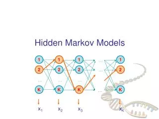
16. Hidden Markov model • HMM = probabilistic observation of Markov chain • Another special kind of Bayesian network • Siform a Markov chain as before, but states are unobserved • Instead, yi (dependent on Si) are observed • Generative viewpoint: state Si “emits” symbol yi • yi do not form a Markov chain (= do not satisfy Markov property)They exhibit more complex (and long-range) dependencies S1 S2 S3 S4 S5 S6 S7 S8 … y1 y2 y3 y4 y5 y6 y7 y8 …

17. Hidden Markov model • Notation above emphasizes relation to Bayesian networks • Different graph notation, emphasizing “transition probabilities” P(Si|Si-1). E.g. in the case Si {A,B,C,D}:Notes: • “Emission probabilities” P( yi | Si ) not explicitly represented • Advance from i to i+1 also implicit • Not all arrows need to be present (prob = 0) S1 S2 S3 S4 S5 S6 S7 S8 … y1 y2 y3 y4 y5 y6 y7 y8 … A B C D

18. Pair Hidden Markov model y1 y2 y3 y4 y5 S11 S21 S31 S41 S51 … z1 S12 S22 S23 S24 S25 … z2 S31 S32 S33 S34 S35 … z3

19. Pair Hidden Markov model y1 y2 y3 y4 y5 • States may “emit” a symbol in sequence y, or in z, or both, or neither (“silent” state). • If a symbol is emitted, the associated coordinate subscript increases by one. E.g. diagonal transitions are associated to simultaneous emissions in both sequences. • A realization of the pair HMM consists of a state sequence, with each symbol emitted by exactly one state, and the associated path through the 2D table. (A slightly more general viewpoint decouples the states and the path; then the hidden variables are the sequence of states S,and a path through the table. In this viewpoint the transitions, not states,emit symbols. The technical term in finite state machine theory is Mealy machine; the standard viewpoint is also known as Moore machine) S11 S21 S31 S41 S51 … z1 S12 S22 S23 S24 S25 … z2 S31 S32 S33 S34 S35 … Normalization: ΣpathspΣsp(1) … sp(N)Σy1…yAΣz1…zBP(sp(1),…,sp(N),y1…yA,z1…zB) = 1 N = N(p) = length of path z3

20. Inference in HMMs So HMMs can describe complex (temporal, spatial) relationships in data. But how can we use the model? • A number of (efficient) inference algorithms exist for HMMs: • Viterbi algorithm: most likely state sequence, given observables • Forward algorithm: likelihood of model given observables • Backward algorithm: together with Forward, allows computation of posterior probabilities • Baum-Welch algorithm: parameter estimation given observables

21. Summary of part I • Probabilistic models Observed variables Latent variables: of interest for inference, or nuisance variables Parameters: obtained from training data, or prior knowledge • Bayesian networks independence structure of model represented as a graph • Markov models linear Bayesian network; all nodes observed • Hidden Markov models observed layer, and hidden (latent) layer of nodes efficient inference algorithm (Viterbi algorithm) • Pair Hidden Markov model two observed sequences with interdependencies, determined by an unobserved Markov sequence

22. Part IIExamples of HMMs

23. Detailed example:The Occasionally Crooked Casino Dirk Husmeier’s slides http://www.bioss.sari.ac.uk/staff/dirk/talks/tutorial_hmm.pdf • Slides 1-15 • Recommended reading: Slides 16-23: the Forward and Backward algorithm, and posteriors

24. Applications in computational biology Dirk Husmeier’s slides: http://www.bioss.sari.ac.uk/staff/dirk/talks/tutorial_hmm_bioinf.pdf • Slides 1-8: pairwise alignment • Slides 12-16: Profile HMMs

25. Part IIIPracticals

26. Practical 0: HMMs • What is the interpretation of the probability computed by the Forward (FW) algorithm? • The Viterbi algorithm also computes a probability. How does that relate to the one computed by the FW algorithm? • How do the probabilities computed by FW and Backward algorithms compare? • Explain what a posterior is, either in the context of alignment using an HMM, or of profile HMMs. • Why is the logarithm trick useful for the Viterbi algorithm? Does the same trick work for the FW algorithm?

27. Practical I: Profile HMMs in context

28. Practical I: Profile HMMs in context • Lookup protein sequence of PRDM9 in the UCSC genome browser • Search Intropro for the protein sequence. Look at the ProSite profile and sequence logo. Work out the syntax of the profile (HMMer syntax), and relate the logo and profile. • Which residues are highly conserved? What structural role do these play? Which are not very much conserved? Can you infer that these are less important biologically? • Read PMID: 19997497 (PubMed). What is the meaning of the changed number of zinc finger motifs across species? Relate the conserved and changeable positions in the zinc fingers to the INTERPRO motif. Do these match the predicted pattern? • Read PMID: 19008249 and PMID:20044541. Explain the relationship between the recombination motif and the zinc fingers. What do you think is the cellular function of PRDM9? • Relate the fact that recombination hotspots in Chimpanzee do not coincide with those in human with PRDM9. What do you predict about recombination hotspots in other mammalian species? Why do you think PRDM9 evolves so fast? Background information on motif finding: www.bx.psu.edu/courses/bx-fall04/phmm.ppt http://compbio.soe.ucsc.edu/SAM_T08/T08-query.html

29. Practical II: HMMs and population genetics

30. Practical II: HMMs and population genetics • Read PMID: 17319744, and PMID: 19581452 • What is the difference between phylogeny and genealogy? What is incomplete lineage sorting? • The model operates on multiple sequences. Is it a linear HMM, a pair HMM, or something else? • What do the states represent? How could the model be improved? • Which patterns in the data is the model looking for? Would it be possible to analyze these patterns without a probabilistic model? (Estimate how frequently (per nucleotide) mutations occur between the species considered. What is the average distance between recombinations?) • How does the method scale to more species?

31. Practical III: HMMs and alignment

32. Practical III: HMMs and alignment • PMID: 18073381 • What are the causes of inaccuracies in alignments? • Would a more accurate model of sequence evolution improve alignments? Would this be a large improvement? • What is the practical limit (in terms of evolutionary distance, in mutations/site) on pairwise alignment? Would multiple alignment allow more divergent species to be aligned? • How does the complexity scale for multiple alignment using HMMs, in a naïve implementation? What could you do to improve this? • What is posterior decoding and how does it work? In what way does it improve alignments, compared to Viterbi? Why is this?

33. Practical IV: HMMs and conservation: phastCons

34. Practical IV: HMMs and conservation: phastCons • Read PMID: 16024819 • What is the difference between a phyloHMM and a “standard” HMM? • How does the model identify conserved regions? How is the model helped by the use of multiple species? How is the model parameterized? • The paper uses the model to estimate the fraction of the human genome that is conserved. How can this estimate be criticized? • Look at a few protein-coding genes, and their conservation across mammalian species, using the UCSC genome browser. Is it always true that (protein-coding) exons are well conserved? Can you see regions of conservation outside of protein-coding exons? Do these observations suggest that the model is inaccurate? • Read PMID: 19858363. Summarize the differences of approaches of the new methods and the “old” phyloHMM.

35. Practical V: Automatic code generation for HMMs

36. Practical V: Automatic code generation for HMMs • http://www.well.ox.ac.uk/~gerton/Gulbenkian/HMMs and alignments.doc. Skip sections 1-3. Implementing the various algorithms for HMMs can be hard work, particularly when a reasonable efficiency is required. Library implementations are however neither fast nor flexible enough. This practical demonstrates a code generator that takes the pain out of working with HMMs. This practical takes you through an existing alignment HMM, and modifies it to identify conserved regions (àla phastCons) Requirements: a Linux system, with Java and GCC installed. Experience with C and/or C++ is helpful for this tutorial.