Parallel prefix adders
Parallel prefix adders. Kostas Vitoroulis, 2006. Presented to Dr. A. J. Al-Khalili. Concordia University. Overview of presentation. Parallel prefix operations Binary addition as a parallel prefix operation Prefix graphs Adder topologies Summary. Parallel Prefix Operation.

Parallel prefix adders
E N D
Presentation Transcript
Parallel prefix adders Kostas Vitoroulis, 2006. Presented to Dr. A. J. Al-Khalili. Concordia University.
Overview of presentation • Parallel prefix operations • Binary addition as a parallel prefix operation • Prefix graphs • Adder topologies • Summary
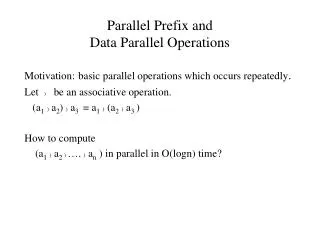
Parallel Prefix Operation Terminology background: • Prefix: The outcome of the operation depends on the initial inputs. • Parallel: Involves the execution of an operation in parallel. This is done by segmentation into smaller pieces that are computed in parallel. • Operation: Any arbitrary primitive operator “ ° ” that is associative is parallelizable • it is fast because the processing is accomplished in a parallel fashion.
Example: Associative operations are parallelizable Consider the logical OR operation: a + b The operation is associative: a + b + c + d = ((( a + b ) + c) + d ) = (( a + b ) + ( c + d)) Serial implementation: Parallel implementation:
Mathematical Formulation: Prefix Sum this is the unary operator known as “scan” or “prefix sum” • Bn represents the operator being applied to all terms of the vector. • Operator: “ ° ” • Input is a vector: A = AnAn-1 … A1 • Output is another vector: B = BnBn-1 … B1 where B1 = A1 B2 = A1° A2 … Bn = A1° A2 … ° An
Example of prefix sum Consider the vector: A = AnAn-1 … A1 where element Ai is an integer The “*” unary operator, defined as: *A = B With B = BnBn-1 … B1 B1= A1 B2 = A1* A2 B3 = A1* A1* A3 … and ‘ * ’ here is the integer addition operation.
6 6 5 5 4 4 3 3 2 2 1 1 6 6 5 5 4 4 3 3 2 2 1 1 + + + B3 = (A1 + A2) + A3 = 6 + B1 = A1 = 1 B2 = A1 + A2 = 3 B6 = A6 +… +A1 = (A6 + A5) + ((A4+A3) +(A2 +A1)) = 21 + + + + + + + + B6 B6 B5 B5 B4 B4 B3 B3 B2 B2 B1 B1 B6 B6 B5 B5 B4 B4 B3 B3 B2 B2 B1 B1 Example of prefix sum Calculation of *A, where A = 6 5 4 3 2 1 yields: B = *A = 21 15 10 6 3 1 Because the summation is associative the calculation can be done in parallel in the following manner: Parallel implementation versus Serial implementation
Binary Addition This is the pen and paper addition of two 4-bit binary numbers x and y. c represents the generated carries. s represents the produced sum bits. A stageof the addition is the set of x and y bits being used to produce the appropriate sum and carry bits. For example the highlighted bits x2, y2 constitute stage 2 which generates carry c2 and sum s2 . c3 c2 c1 c0 x3 x2 x1 x0 Each stage i adds bits ai, bi, ci-1 and produces bits si, ci The following hold: + y3 y2 y1 y0 s4 s3 s2 s1 s0
Binary Addition The carry ci generated by a stage i is given by the equation: This equation can be simplified to: The “ai” term in the equation being the “alive” bit. The later form of the equation uses an OR gate instead of an XOR which is a more efficient gate when implemented in CMOS technology. Note that: Where ki is the “kill” bit defined in the table above.
Pre-calculation of pi, gi for each stage Calculation of carry ci for each stage. Combine ci and pi of each stage to generate the sum bits si Carry Look Ahead adders The CLA adder has the following 3-stage structure: Final sum.
x0y0 x1y1 x2y2 g0 g1 g2 p2 p0 p1 x1y1 x0y0 x2y2 g1 a1 g0 a0 g2 a2 Carry Look Ahead adders • The pre-calculation stage is implemented using the equations for pi, gi shown at a previous slide: • Alternatively using the “alive” bit: • Note the symmetry when we use the “propagate” or the “alive” bit… We can use them interchangeably in the equations!
g1p1 g0p0 g2p2 Carry generator block c2 c1 c0 Carry Look Ahead adders • The carry calculation stage is implemented using the equations produced when unfolding the recursive equation:
cinp0 c2p3 c1p2 c0p1 s0 s3 s2 s1 Carry Look Ahead adders • The final sum calculation stage is implemented using the carry and propagate bits ci,pi: • If the ‘alive’ bit ai is used the final sum stage becomes more complex as implied by the equations above.
Binary addition as a prefix sum problem. • We define a new operator: “ ° ” • Input is a vector of pairs of ‘propagate’ and ‘generate’ bits: • Output is a new vector of pairs: • Each pair of the output vector is calculated by the following definition:
Binary addition as a prefix sum problem. • Properties of operator “ ° ”: • Associativity (hence parallelization) • Easy to prove based on the fact that the logical AND, OR operations are associative. • With the definition: Gi becomes the carry signal at stage i of an adder. Illustration on next slide. • The operation is idempotent • Which implies
A stage i will generate a carry if gi=aibi and propagate a carry if pi=XOR(ai,bi) Hence for stage i: ci=gi+pici-1 a3 a2 a1 a0 + b3 b2 b1 b0 … The familiar carry bit generating equations for stage i in a CLA adder. Binary Addition as a prefix sum problem.
Addition as a prefix sum problem. • Conclusion: • The equations of the well known CLA adder can be formulated as a parallel prefix problem by employing a special operator “ ° ”. • This operator is associative hence it can be implemented in a parallel fashion. • A Parallel Prefix Adder (PPA) is equivalent to the CLA adder… The two differ in the way their carry generation block is implemented. • In subsequent slides we will see different topologies for the parallel generation of carries. Adders that use these topologies are called Parallel Prefix Adders.
Straight forward as in the CLA adder Pre-calculation of Pi, Gi terms Prefix graphs can be used to describe the structure that performs this part. Calculation of the carries. This part is parallelizable to reduce time. Simple adder to generate the sum Straight forward as in the CLA adder Parallel Prefix Adders • The parallel prefix adder employs the 3-stage structure of the CLA adder. The improvement is in the carry generation stage which is the most intensive one:
Calculation of carries – Prefix Graphs The components usually seen in a prefix graph are the following: processing component:buffer component:
(p2, g2) (p8, g8) (p7, g7) (p6, g6) (p5, g5) (p4, g4) (p3, g3) (p1, g1) c8 c7 c6 c5 c4 c3 c2 c1 Prefix graphs for representation of Prefix addition • Example: serial adder carry generation represented by prefix graphs
Key architectures for carry calculation: • 1960: J. Sklansky – conditional adder • 1973: Kogge-Stone adder • 1980: Ladner-Fisher adder • 1982: Brent-Kung adder • 1987: Han Carlson adder • 1999: S. Knowles Other parallel adder architectures: • 1981: H. Ling adder • 2001: Beaumont-Smith
(p2, g2) (p8, g8) (p7, g7) (p6, g6) (p5, g5) (p4, g4) (p3, g3) (p1, g1) c8 c7 c6 c5 c4 c3 c2 c1 1960: J. Sklansky – conditional adder • The Sklansky adder has: • Minimal depth • High fan-out nodes
1973: Kogge-Stone adder (p8, g8) (p7, g7) (p6, g6) (p5, g5) (p4, g4) (p3, g3) (p1, g1) (p2, g2) c8 c7 c6 c5 c4 c3 c2 c1 • The Kogge-Stone adder has: • Low depth • High node count (implies more area). • Minimal fan-out of 1 at each node (implies faster performance).
1980: Ladner-Fischer adder (p2, g2) (p8, g8) (p7, g7) (p6, g6) (p5, g5) (p4, g4) (p3, g3) (p1, g1) c8 c7 c6 c5 c4 c3 c2 c1 • The Ladner-Fischer adder has: • Low depth • High fan-out nodes • This adder topology appears the same as the Schlanskly conditional sum adder. Ladner-Fischer formulated a parallel prefix network design space which included this minimal depth case. The actual adder they included as an application to their work had a structure that was slightly different than the above.
1982: Brent-Kung adder (p2, g2) (p8, g8) (p7, g7) (p6, g6) (p5, g5) (p4, g4) (p3, g3) (p1, g1) c8 c7 c6 c5 c4 c3 c2 c1 • The Brent-Kung adder is the extreme boundary case of: • Maximum logic depth in PP adders (implies longer calculation time). • Minimum number of nodes (implies minimum area).
1987: Han Carlson adder • The Han-Carlson adder combines the Brent-Kung and Kogge-Stone structures into a hybrid structure. • Efficient • Suitable for VLSI implementation.
1999: S. Knowles • Knowles proposed adders that trade off: • Depth, interconnect, area. • These adders are bound by the Lander-Fischer (minimum depth) and Brent-Kung (minimum fanout) topologies. Brent-Kung topology (Minimum fan-out) Knowles topologies (Varied fan-out at each level ) Ladner-Fischer topology (Minimum depth, high fanout)
An interesting taxonomy: • Harris[2003] presented an interesting 3-D taxonomy of the adders presented so far. • Each axis represents a characteristic of the adders: • Fanout • Logic depth • Wire connections • He also proposed the following structure:
1981: H. Ling adder Ling Adders are a different family of adders. They can still be formulated as prefix adders. Ling adders differ from the “traditional” PP adders in that: • They are based on a different set of equations. • The new set of equations introduces the following tradeoffs: Precalculation of Pi, Gi terms is based on morecomplex equations Calculation of the carries is based on simpler equations Final addition stage is more complex
2001: Beaumont-Smith (p2, g2) (p8, g8) (p7, g7) (p6, g6) (p5, g5) (p4, g4) (p3, g3) (p1, g1) c8 c7 c6 c5 c4 c3 c2 c1 • The Beaumont-Smith adders incorporate nodes that can accept more than a pair of inputs and produce the carry calculation. • These ‘higher valency’ nodes are optimized circuits for a specific technology (CMOS). • The above topology is a Beaumont-Smith tree based on the Kogge-Stone architecture
Summary (1/3) • The parallel prefix formulation of binary addition is a very convenient way to formally describe an entire family of parallel binary adders.
Summary (2/3) • A parallel prefix adder can be seen as a 3-stage process: • There exist various architectures for the carry calculation part. • Trade-offs in these architectures involve the • area of the adder • its depth • the fan-out of the nodes • the overall wiring network. Pre-calculation of Pi, Gi terms Calculation of the carries. Simple adder to generate the sum
Summary (3/3) • Variations of parallel adders have been proposed. These variations are based on: • Modifying the carry generation equations and reformulating the prefix definition (Ling) • Restructuring the carry calculation trees based by optimizing for a specific technology (Beaumond-Smith) • Other optimizations.
References: Beaumont-Smith, Cheng-Chew Lim, “Parallel Prefix Adder Design”, IEEE, 2001 Han, Carlson, “Fast Area-Efficient VLSI Adders, IEEE, 1987 Dimitrakopoulos, Nikolos, “High-Speed Parallel-Prefix VLSI Ling Adders”, IEEE 2005 Kogge, Stone, “A Parallel Algorithm for the Efficient solution of a General Class of Recurrence equations”, IEEE, 1973 Simon Knowles, “A Family of adders”, IEEE, 2001 Ladner, Fischer, “Parallel Prefix Computation”, ACM, 1980 Brent, Kung, “A regular Layout for Parallel Adders”, IEEE, 1982 H. Ling, “High-Speed Binary Adder”, IBM J. Res. And Dev., 1980 J. Sklansky, “Conditional-Sum Addition Logic”, IRE transactions on computers, 1960 D. Harris, “A Taxonomy of Parallel Prefix Networks”, IEEE, 2003