Scanning Probe Microscope - SPM -
אוניברסיטת בן-גוריון בנגב הפקולטה למדעי ההנדסה המחלקה להנדסת חשמל ומחשבים. Scanning Probe Microscope - SPM -. Present Rony Levin Email levinbr@ee.bgu.ac.il Course Nanotechnology Number 361-2-0826 Lecturer Dr. Ilan Shalish. Agenda. Terms Definition Historical Overview SPM Overview


Scanning Probe Microscope - SPM -
E N D
Presentation Transcript
אוניברסיטת בן-גוריון בנגב הפקולטה למדעי ההנדסה המחלקה להנדסת חשמל ומחשבים Scanning Probe Microscope - SPM - Present Rony Levin Email levinbr@ee.bgu.ac.il Course Nanotechnology Number 361-2-0826 Lecturer Dr. Ilan Shalish
Agenda • Terms Definition • Historical Overview • SPM Overview • SPM Software • STM Overview • AFM Overview • Summary
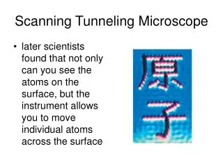
Terms Definition MicroscopyμΙκροσ-small, σκοποσ– see Scanning Probe Microscopy (SPM) is a branch of microscopy that forms images of surfaces using a physical probe that scans the specimen Artifact is any perceived distortion or other data error caused by the instrument of observation Cantilever is a beam supported on only one end from wikipedia
Terms Definition Input transducer or sensor Convert nonelectrical signal to electrical one Output transducer or actuator Convert electrical signal to nonelectrical one Piezoceramic Ceramic that convert electrical field to mechanical deformation and vice versa Piezoelectric properties are time-depended
Acronyms SPM Scanning Probe Microscope STM Scanning Tunneling Microscope AFM Atomic Force Microscope SFM Scanning Force Microscope FFM Force-Modulated AFM LFM Lateral Force Microscope MFM Magnetic Force Microscope SThM Scanning Thermal Microscope EFM Electrical Force Microscope
Historical Overview • 1981 STM was developed by Binnig and Rohrer, IBM, Zurich • 1986 AFM was developed by Binnig, Quarter and Gerber • 1988 Commercial SPM available • 1990 Analog electronics replaced by digital • 1990 Software for SPM based Microsoft Windows developed • from 1990 SPM market wake up Agilent Technologies, nanoScience …
SPM Physical ModelThe Blind Mouse Computer Actuator Probe Sensor Sample
Blind Mouse Operational Principle The blind mouse can’t see the object (sample), but using the stick (probe), he can scan it. Arm skin (sensor) send the received from the probe information to the brain (computer), the computer “see” the picture, if it need receive additional information about the sample (decision done using feedback), it send requirement to arm muscle (actuator), arm carefully moves the probe to required coordinate and vice versa
SPM Operational Principle All of the SPM techniques are based upon scanning a probe (typically called the tip, since it literally is a sharp metallic tip) just above a surface whilst between scanned surface and probe exist interaction The nature of this chosen interaction defines a device accessory to this or that type within the family of Scanning Probe Microscope The information on a surface is taken by fixing (by means of feedback system) or monitoring of interaction of a probe and the sample
SPM Operational Principle We will present scanning probe microscopes based on two kind of iteration • Iteration is electrical current STM • Iteration is atomic force AFM/SFM In general, as mentioned, SPM have two modes, defined by tip movement over the surface • Fixed probe Z coordinate, iteration or parameter depended on iteration monitoring • Fixed iteration, height change monitoring
STM Operational Principle from site
Potential Barrier Schematics V is bias voltage EF is Fermi level
Step Potential Barrier Schrödinger time invariant equation
Transfer Matrix General solution Using C1 connectivity
Transfer Matrix Transfer Matrix Definition Now it can be written more simple
Transfer Matrix We received very powerful mathematical tool. Using this algorithm and Matlab we can solve complicated potential barriers
Tunneling-Summary Received result is not so suitable for classical physics theory, were electron position defined as “to be or not to be” In quantum mechanics theory electron position defined as “may be” and appropriate number from 0 to 1 that describe the chance of electron to be in some coordinate. Summarizing all the electrons over all energy levels, that can pass the barrier, will receive tunneling current expression
Distance Sensitivity What happened if current will be changed, how mach it will affect the distance? Assume that K=4 eV, current precision is 2%
Feedback control signal Control System feedback signal error reference
Calibration • Error as result of non orthogonal axes and reference point definition • Error as result of probe geometric shape • Error as result of sensor sensitivity In order to avoid measurement errors depended on setup, mandatory to perform pre measurement system calibration
AFM Operational Principle from site
Thank You for Attention
Stam • SPM