Download
1 / 29
290 likes | 516 Vues
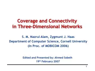
Coverage and Connectivity in Three-Dimensional Networks. S. M. Nazrul Alam, Zygmunt J. Haas Department of Computer Science, Cornell University (In Proc. of MOBICOM 2006). Edited and Presented by: Ahmed Sobeih 19 th February 2007. Motivation. Conventional network design

E N D
Coverage and Connectivity in Three-Dimensional Networks S. M. Nazrul Alam, Zygmunt J. Haas Department of Computer Science, Cornell University (In Proc. of MOBICOM 2006) Edited and Presented by: Ahmed Sobeih 19th February 2007
Motivation • Conventional network design • Almost all wireless terrestrial network based on 2D • In cellular system, hexagonal tiling is used to place base station for maximizing coverage with fixed radius • In Reality: Distributed over a 3D space • Length and width are not significantly larger than height • Deployed in space, atmosphere or ocean • Underwater acoustic ad hoc and sensor networks • Army: unmanned aerial vehicles with limited sensing range or underwater autonomous vehicles for surveillance • Climate monitoring in ocean and atmosphere
Motivation (cont’d) • Need to address problems in 3D • Problems in 3D usually more challenging than in 2D • Today’s paper: coverage and connectivity in 3D • Authors have another work on topology control and network lifetime in 3D wireless sensor networks • http://www.cs.cornell.edu/~smna/
Problem Statement • Assumptions • All nodes have the same sensing range and same transmission range • Sensing range R≤ transmission range • Sensing is omnidirectional, sensing region is sphere of radius R • Boundary effects are negligible: R<<L, R<<W, R<<H • Any point in 3D must be covered by (within R of) at least one node • Free to place a node at any location in the network • Two goals of the work • 1: Node Placement Strategy) Given R, minimize the number of nodes required for surveillance while guaranteeing 100% coverage. Also, determine the locations of the nodes. • 2: Minimum ratio) between the transmission range and the sensing range, such that all nodes are connected to their neighbors
Roadmap of the paper • Proving optimality in 3D problems • Very difficult, still open for the centuries! • E.g., Kepler’s conjecture (1611) and proven only in 1998! • E.g., Kelvin’s conjecture (1887) has not been proven yet! • Instead of proving optimality • Show similarity between our problem and Kelvin’s problem. • Use Kelvin’s conjecture to find an answer to the first question. • Any rigorous proof of our conjecture will be very difficult. • Instead of giving a proof: • provide detailed comparisons of the suggested solution with three other plausible solutions, and • show that the suggested solution is indeed superior.
Outline • Motivation • Problem Statement • Raodmap of the Paper • Preliminaries • Space-Filling Polyhedron • Kelvin’s Conjecture • Voronoi Tessellation • Analysis • Conclusion
Space-Filling Polyhedron • Polyhedron • is a 3D shape consisting of a finite number of polygonal faces • E.g., cube, prism, pyramid • Space-Filling Polyhedron • is a polyhedron that can be used to fill a volume without any overlap or gap (a.k.a, tessellation or tiling) • In general, it is not easy to show that a polyhedron has the space-filling property In 350 BC, Aristotle claimed that the tetrahedron (4{3}) is space-filling, but his claim was incorrect. The mistake remained unnoticed until the 16th century! Cube (6{4}) is space-filling
Why Space-Filling?! • How is our problem related to space-filling polyhedra? • Sensing region of a node is spherical • Spheres do NOT tessellate in 3D • We want to find the space-filling polyhedron that “best approximates” a sphere. • Once we know this polyhedron: • Each cell is modeled by that polyhedron (for simplicity), where the distance from the center of a cell to its farthest corner is not greater than R • Number of cells required to cover a volume is minimized • This solves our first problem • The question still remains: What is this polyhedron?!
Kelvin’s Conjecture • In 1887, Lord Kelvin asked: • What is the optimal way to fill a 3D space with cells of equal volume, so that the surface area is minimized? Lord Kelvin (1824 - 1907) • Essentially the problem of finding a space-filling structure having the highest isoperimetric quotient: • 36 π V2 / S3 • where V is the volume and S is the surface area • Sphere has the highest isoperimetric quotient = 1 • Kelvin’s answer: 14-sided truncated octahedron having a very slight curvature of the hexagonal faces and its isoperimetric quotient = 0.757
Truncated Octahedron Truncated Octahedron (6{4} + 8{6}) is space-filling. The solid of edge length a can be formed from an octahedron of edge length 3a via truncation by removing six square pyramids, each with slant height and base = a Octahedron (8{3}) is NOT space-filling Truncated Octahedra tessellating space
Voronoi Tessellation (Diagram) • Given a discrete set S of points in Euclidean space • Voronoi cell of point c of S: • is the set of all points closer to c than to any other point of S • A Voronoi cell is a convex polytope (polygon in 2D, polyhedron in 3D) • Voronoi tessellation corresponding to the set S: • is the set of such polyhedra • tessellate the whole space • The paper assumes each Voronoi cell is identical Voronoi Diagram Hexagonal tessellation of a floor. All cells are identical.
Analysis • Total number of nodes for 3D coverage • Simply, ratio of volume to be covered to volume of one Voronoi cell • Minimizing no. of nodes by maximizing the volume of one cell V • With omnidirectional antenna: sensing range R sphere • Radius of circumsphere of a Voronoi cell ≤ R • To achieve highest volume, radius of circumsphere = R • Volume of circumsphere of each Voronoi cell: 4πR3/3 • Find space-filling polyhedron that has highest volumetric quotient; i.e., “best approximates” a sphere. • Volumetric quotient, q: 0 ≤ q ≤ 1 • For any polyhedron, if the maximum distance from its center to any vertex is R and the volume of the polyhedron is V, then the volumetric quotient is,
Analysis • Similarity with Kelvin’s Conjecture • Kelvin’s: find space-filling polyhedron with highest isoperimetric quotient • Sphere has the highest isoperimetric quotient = 1 • Ours: find space-filling polyhedron with highest volumetric quotient • Sphere has the highest volumetric quotient = 1 • Both problems: find space-filling polyhedron “best approximates” the sphere • Among all structures, the following claims hold: • For a given volume, sphere has the smallest surface area • For a given surface area, sphere has the largest volume • Claim/Argument: • Consider two space-filling polyhedrons: P1 and P2 such that VP1 = VP2 • If SP1 < SP2, then P1 is a better approximation of a sphere than P2 • If P1 is a better approximation of a sphere than P2, then P1 has a higher volumetric quotient than P2 • Conclusion: Solution to Kelvin’s problem is essentially the solution to ours!
Analysis: choice of other polyhedra • Cube • Simplest, only regular polyhedron tessellating 3D space • Hexagonal prism • 2D optimum: hexagon, 3D extension, Used in [8] • Rhombic dodecahedron • Used in [6] • Analysis • Compare truncated octahedron with these polyhedra • Show that the truncated octahedron has a higher volumetric quotient, hence requires fewer nodes
Analysis: volumetric quotient 1 • Cube • Length: a • Radius of circumsphere = R = • Volumetric quotient: • Given R, compute a • Sensing range: R = • a= =1.1547R
Analysis: volumetric quotient 2 • Hexagonal Prism • Length: a, height: h • Volume = area of base * height • Radius of circumsphere = R = • Volumetric quotient • Optimal h: Set first derivative of volumetric quotient to zero • Optimum volumetric quotient,
Analysis: volumetric quotient 3 • Rhombic dodecahedron • 12 rhombic face • Length: a • Radius of circumsphere: a • Volumetric quotient
Analysis: volumetric quotient 4 • Truncated Octahedron • 14 faces, 8 hexagonal, 6 square space • Length: a • Radius of circumsphere: • Volumetric quotient
Analysis: Comparison Inverse proportion
Analysis: Placement strategies • Node placement • Where to place the nodes such that the Voronoi cells are our chosen space-filling polyhedrons? • Choose an arbitrary point (e.g., the center of the space to be covered): (cx, cy, cz). Place a node there. • Idea: Determine the locations of other nodes relative to this center node. • New coordinate system (u, v, w). Nodes placed at integer coordinates of this coordinate system. • Input to the node placement algorithm: • (cx, cy, cz) • Sensing range R • Output of the node placement algorithm: • (x, y, z) coordinates of the nodes • Distance between two nodes (needed to calculate transmission range. Prob. 2)
Analysis: Placement strategies 1 • Cube • Recall: Radius of circumsphere = R = • Unit distance in each axis = a = • (u, v, w) are parallel to (x, y, z) • A node at (u1, v1, w1) in the new coordinate system should be placed in the original (x, y, z) coordinate system at • Distance between two nodes
Analysis: Placement strategies 2 • Hexagonal Prism • Recall: , R = = • Hence, a = , h = • New coordinate system (u, v, w): • v-axis is parallel to y-axis. • Angle between u-axis and x-axis is 300 • w-axis is parallel to z-axis • Unit distance along v-axis = Unit distance along u-axis = • Unit distance along z-axis = h =
Analysis: Placement strategies 2 • Hexagonal Prism (cont’d) • A node at (u1, v1, w1) in the new coordinate system should be placed in the original (x, y, z) coordinate system at • Distance between two nodes =
Analysis: Placement strategies 3 • Rhombic Dodecahedron • Unit distance along each axis: • New coordinate system placed in the original coordinate system at (3) • Distance between two nodes
Analysis: Placement strategies 4 • Truncated octahedron • Unit distance in both u and v axes: , w axis: • New coordinate system placed in the original coordinate system at (4) • Distance between two nodes
Analysis: Transmission vs. Sensing Range • Required transmission range • To maintain connectivity among neighboring nodes • Depend on the choice of the polyhedron
Simulation • Graphical output of placing node • http://www.cs.cornell.edu/~smna/3DNet/ • Cube: eq.(1) • Hexagonal prism: eq.(2) • Rhombic dodecahedron: eq.(3) • Truncated octahedron: eq.(4)
Conclusion • Performance comparison • Truncated octahedron: higher volumetric quotient (0.683) than others(0.477, 0.367) • Required much fewer nodes (others more than 43%) • Maintain full connectivity • Optimal placement strategy for each polyhedron • Truncated octahedron: requires the transmission range to be at least 1.7889 times the sensing range • Further applications • Fixed: initial node deployment • Mobile: dynamically place to desired location • Node ID: u,v,w coordination location-based routing protocol
Questions? Thank You!