
Location Determination
E N D
Presentation Transcript
Location Determination Framework and Technologies
Meaning of Location • Three Dimensional Space • Reference Coordinate System • Global – GPS • Local • Application Specific • Multiple References • Ability to Map • Notation
Location Uses • All levels of accuracies have applications • Outdoors • Navigation • Automobiles/ Road Vehicles • Aircrafts • Boats/Ships • Personal – walking/jogging/running • Targetting • Finding Hospitals/Gas Stations…. • Indoors • Advertising • Finding … • System based vs. device based
How • Benchmarks • Known locations (Accuracy?) • Unknown Location WRT the location of Benchmarks • What Form ?? • Physical, marked locations • Location of devices • What do I measure?? • Proximity • Distance • Some function of distance • Direction • Some function of direction • How many measurements • 3 • 4 • Use Geometry • Triangulation • Trilateration
Desirable Features • In Doors and Out Doors operation • Independent of GPS • Rapidly Deployable • Agnostic to Frequency Band or Protocol • Accurate • Scalable • …
Proximity • Detect the presence close to a known location • RFID • Passive • Read by putting in a field of RF and reading the scatter pattern • Inventory Control • EZPass • Active • iBeacon • Using low power Bluetooth • Estimotes • …. • How does Passive RFID approach compare with barcodes? • FingerPrinting Based approach in WiFi Field
RF Field Based - WiFi • AP – Generate Beacons 100 ms • Can measure signal Strength • RSSI – Received Signal Strength Indicator • Included in spec to support handovers. • RSSI – Relative scale or dbm • Most devices now report dbm • Range (-50 to -90 dbm) • Integer values only
Problem Formulation • K Access Points • Signal Field Where S is k dimensional vector and X is the location vector. • Problem – The signal strength of K APs is measured by a device as signal vector S. Determine the location X where the device is • Issues: • Is S an invertible function? • Does S have a closed form? • Is S deterministic or do the measurements vary with time
Signal Function • Closed Form • Maxwell Equations • Affected by • Decay • Reflections • Refraction • Diffusion • Scattering • Some Approximations have been attempted • Outdoor – Cellular Phone • Accuracies ~200 meters • Indoor – WiFi • Accuracies 5-10 meters • What should be K, the number of signal generators – APs. • Most WiFideployment is for supporting networking access and not for location. • At a location one can only hear a small number of APs. • There are ~4500 APs on campus. How do we efficiently handle this 4500 dimensional function?
Stochastic nature of Signals • Repeated measurements vary when nothing has changed • There is some correlation among samples • Signal Vector has to be treated as a stochastic vector • As it is reasonable to assume that all APs operate independently the signals from them can be treated as independent random variables. • Analytical models require the modeling of the randomness
FingerPrinting • We can estimate the joint probability distribution of the signal vector by empirical measurements • Discretize X and make measurements of S at known locations – a grid in X space • Treat the measurement points as benchmark points • Find the benchmark point closest to the device signal vector in signal space • May refine the location by determining a few closest benchmark points and interpolating
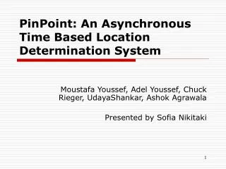
H O R U S H O R U S Horus: A WLAN-Based Indoor Location Determination System Moustafa Youssef
WLAN Location Determination (Cont’d) • Signal strength= f(distance) • Does not follow free space loss • Use lookup table Radio map • Radio Map: signal strength characteristics at selected locations
(xi, yi) (x, y) WLAN Location Determination (Cont’d) [-50, -60] • Offline phase • Build radio map • Radar system: average signal strength • Online phase • Get user location • Nearest location in signal strength space (Euclidian distance) 5 [-53, -56] 13 [-58, -68]
Horus Goals • High accuracy • Wider range of applications • Energy efficiency • Energy constrained devices • Scalability • Number of supported users • Coverage area
Sampling Process • Active scanning • Send a probe request • Receive a probe response
Signal Strength Characteristics • Temporal variations • One access point • Multiple access points • Spatial variations • Large scale • Small scale
Testbeds • FLA • 3rd floor, 8400 Baltimore Ave • 39 feet by 118 feet • LinkSys/Cisco APs • 6 APs (4 on avg.) • 110 locations • 7 feet apart • Linux (kernel 2.5.7) • A.V. William’s • 4th floor, AVW • 224 feet by 85.1 feet • UMD net (Cisco APs) • 21 APs (6 on avg.) • 172 locations • 5 feet apart • Windows XP Prof. Orinoco/Compaq cards
Horus Components • Basic algorithm [Percom03] • Correlation handler [InfoCom04] • Continuous space estimator [Under] • Locations clustering [Percom03] • Small-scale compensator [WCNC03]
Basic Algorithm:Mathematical Formulation • x: Position vector • s: Signal strength vector • One entry for each access point • s(x) is a stochastic process • P[s(x), t]: probability of receiving s at x at time t • s(x) is a stationary process • P[s(x)] is the histogram of signal strength at x
Basic Algorithm:Mathematical Formulation • Argmaxx[P(x/s)] • Using Bayesian inversion • Argmaxx[P(s/x).P(x)/P(s)] • Argmaxx[P(s/x).P(x)] • P(x): User history
Basic Algorithm • Offline phase • Radio map: signal strength histograms • Online phase • Bayesian based inference
(xi, yi) (x, y) WLAN Location Determination (Cont’d) -40 -60 -80 P(-53/L1)=0.55 [-53] P(-53/L2)=0.08 -40 -60 -80
Basic Algorithm: Results • Accuracy of 5 feet 90% of the time • Slight advantage of parametric over non-parametric method • Smoothing of distribution shape
Correlation Handler • Need to average multiple samples to increase accuracy • Independence assumption is wrong
Correlation Handler:Autoregressive Model • s(t+1)=.s(t)+(1- ).v(t) • : correlation degree • E[v(t)]=E[s(t)] • Var[v(t)]= (1+ )/(1- ) Var[s(t)]
Correlation Handler: Averaging Process • s(t+1)= .s(t)+(1- ).v(t) • s ~ N(0, m) • v ~ N(0, r) • A=1/n (s1+s2+...+sn) • E[A(t)]=E[s(t)]=0 • Var[A(t)]= m2/n2 { [(1- n)/(1- )]2 + n+ 1- 2 *(1- 2(n-1))/(1- 2) }
Correlation Handler: Results • Independence assumption: performance degrades as n increases • Two factors affecting accuracy • Increasing n • Deviation from the actual distribution
Continuous Space Estimator • Enhance the discrete radio map space estimator • Two techniques • Center of mass of the top ranked locations • Time averaging window
Center of Mass: Results • N = 1 is the discrete-space estimator • Accuracy enhanced by more than 13%
Time Averaging Window: Results • N = 1 is the discrete-space estimator • Accuracy enhanced by more than 24%
Horus Components • Basic algorithm • Correlation handler • Continuous space estimator • Small-scale compensator • Locations clustering
Small-scale Compensator • Multi-path effect • Hard to capture by radio map (size/time)
Small-scale Compensator: Small-scale Variations AP1 AP2 • Variations up to 10 dBm in 3 inches • Variations proportional to average signal strength
Small-scale Compensator:Perturbation Technique • Detect small-scale variations • Using previous user location • Perturb signal strength vector • (s1, s2, …, sn) (s1d1, s2d2, …, sndn) • Typically, n=3-4 • di is chosen relative to the received signal strength
Small-scale Compensator: Results • Perturbation technique is not sensitive to the number of APs perturbed • Better by more than 25%
Horus Components • Basic algorithm • Correlation handler • Continuous space estimator • Small-scale compensator • Locations clustering
Locations Clustering • Reduce computational requirements • Two techniques • Explicit • Implicit
S=[-45, -60, -70, -80, -86] q=3 Locations Clustering: Explicit Clustering • Use access points that cover each location • Use the q strongest access points S=[-60, -45, -80, -86, -70]
Locations Clustering:Results- Explicit Clustering • An order of magnitude enhancement in avg. num. of oper. /location estimate • As q increases, accuracy slightly increases
Locations Clustering: Implicit Clustering S=[-60, -45, -80, -86, -70] • Use the access points incrementally • Implicit multi-level clustering S=[-45, -60, -70, -80, -86] S=(-45, -60, -70, -80, -86)
Locations Clustering:Results- Implicit Clustering • Avg. num. of oper. /location estimate better than explicit clustering • Accuracy increases with Threshold