Download
1 / 49
500 likes | 637 Vues
This guide provides an overview of various data visualization techniques in R, including plotting basic graphs such as line plots, scatter plots, and bar charts. Learn how to customize your plots with titles, labels, and colors, and create multiple plots in one layout. Explore how to save your graphs in different formats, and visualize distributions using histograms and QQ plots. The guide emphasizes the use of R's built-in functions to enhance the visual presentation of your data, ensuring effective communication of information.

E N D
X<-c(1:25) • Y<-X^2
Main and labels • plot(X,Y,main="Fuelconsumption for cars", xlab="weight of car",ylab="cl per mile",cex.lab=1.5, sub ="source: Källa",cex.main=2) • Xlab creates label for X • Ylab creates label for Y • Sub creates subtitle • cex.lab decides size of text on labels • cex.main decides size of text on header
plot(X,Y) • It is problematic to use function ”title” for writing labels because it writes over original labels • title(main="Fuelconsumption for cars", xlab="weight of car",ylab="cl per mile”)
par(mfrow=c(2,2)) #Multiple graphs in one picture. Choose your own dimensions i with • # To illustrate different points is given by pch • X<-c(1,2,3,4,5) • Y<-X^2 • plot(X,Y, pch=1, main=" turned squares") • plot(X,Y, pch=2, main ="triangel") • plot(X,Y, pch=3,main="plus") • plot(X,Y, pch=4,main="X")
Get your own symbols • plot(X,Y, pch="*",main=”starplot") • Or choose your own string • z<-c("H", "Å", "K", "A", "N") • plot(X,Y, pch=z,main="Nameplot")
Text instead of points • data<-read.table("Rstudy.txt",header=TRUE) • attach(data) • plot(beer,wine,type="n") • text(beer,wine,country)
Regression • library(foreign) • lnu91<-read.dta("lnu91.dta") • gender<-lnu91$y10 • wage<-lnu91$y472 • age<-lnu91$y11 • lnu<-data.frame(wage,age,gender) • lnu<-na.omit(lnu) • rm(lnu91) • rm(age,wage,gender) • lnu<-subset(lnu, age<67 & wage<300&wage>0) • attach(lnu) • plot(age,log(wage)) • abline (lm(log(wage) ~ age )) #regressionslinje
Show different subgroups plot(age,wage,col=as.numeric(gender)) • Col sets colour. • R has over 650 different colours. Get a list with colors() • plot(age,wage,col=as.numeric(gender),pch=as.numeric(gender)) • Pch sets different characters • Use replace to get the ”right” number
Saving graphs • In pdf • pdf("myfile.pdf") • plot(X,Y)…………… • dev.off() • In postscript • postscript("myfile.eps“, horizontal=FALSE) (A4) • plot(x,y) …………… • dev.off() • In JPEG • jpeg("myfile.jpeg") • plot(X,Y)…… • dev.off() • Similar is available for png and bmp
Drawing functions • curve(atan(x),-25,25) • z<-seq(-25,0,0.01) • a <-seq(0,25,0.01) • z2<-c(rep(-1.57,length(z))) • a2<-c(rep(1.57,length(a))) • lines(a,a2,lty=2) • lines(z,z2,lty=2) • title(main="arctan")
Plotting normaldistribution • For educationalpurposes (Picture on next slide) • nx<-seq(-3,3,0.01) • N<-dnorm(nx) • plot(nx,N,type="l") • polygon(c(nx[nx>=1.96],1.96),c(N[nx>=1.96],N[nx==3]),col="pink") • arrows(2.6,0.1,2.5,0.01) • text(2.65, .12,"2.5 %")
Histogram • hist(wage) • hist(wage,breaks=40) • hist(wage,breaks=40,freq=FALSE) • hist(wage,breaks=seq(0,300,20)) • It is possible to cheat R with!!! • hist(wage,breaks=c(0,25,50,75,100,125,500),freq=TRUE) • With normal distribution curve • hist(wage,breaks=40, prob=TRUE) • x <- seq(0,400,1) • lines(x,dnorm(x,mean(wage),sd(wage)))
Normal distributed? • qqnorm(wage) • qqline(wage) • qqnorm(log(wage)) • qqline(log(wage))
Barchart • occu<-c(rep("Steelworker",320),rep("Chef",250),rep("Gardner",200),rep("Constructionworker",130)) • barplot(occu) #doesn’t work • occ.table <- table(occu) • farger<-c("gold1", "gold2", "gold3", "gold4 ") #Chooses a string with colournames) • barplot(occ.table,col=farger) • barplot(occ.table,col=farger) • barplot(occ.table,col=farger,horiz=TRUE,main="occupations",xlab="Frequency") • Source for further barcharts issuses • http://ww2.coastal.edu/kingw/psyc480/html/barplot_tips.html
Barcharts continuing • Gender<-rep(c("man","man","woman","woman","woman","man","man","man","woman","man"),time=90) #creates Gender variabel • Occ.table2<-table(Gender,occu) • Occ.table2<-table(Gender,occu) #legend gives ”box” • barplot(Occ.table2,legend=T,ylim=c(0,400)) • # Bedside gives pairwise, ylim sets range of y • barplot(Occ.table2,legend=T,ylim=c(0,250),beside=T)
Piechart • seq(0.4,1.0,length=4) • 0.4 0.6 0.8 1.0 • pie(occ.table, col=gray(seq(0.4,1.0,length = 4))) • Radius decides how big radius is to be • Too change background colour: • par(bg="pink") # sets to pink until changed • pie(occ.table, col=gray(seq(0.4,1.0,length = 4)))
Different sizes of the symbols • Different sizes of the symbols is given by • Q<-c(7,3,4,5,12) #gives different sizes for the coordinates • symbols(X,Y,squares = Q) • # Färglägger • W<-c(2,3,6,3,6) • symbols(X,Y,squares = Q,fg=W) • symbols(X,Y,squares = Q,bg=W) • symbols(X,Y,squares = Q,bg=W,fg=W) • Country<-c ("Sweden", "Iceland", "Denmark", "Finland", "Norway") • text(X,Y,Country)
Different kinds of lines • par(mfrow=c(2,1)) • plot(X,Y, type=“l”,lty=0, main= “blank line”) • plot(X,Y, type=“l”,lty=1, main= “solid line”) • plot(X,Y, type=”l”,lty=2, main= “dashed line”) • plot(X,Y, type=”l”,lty=3, main= “dotted line”) • plot(X,Y, type=”l”,lty=4, main= “dotdash line”) • plot(X,Y, type=”l”,lty=5, main= “longdash line”) • plot(X,Y, type=”l”,lty=6, main= “twodash line”)