Mathematical Modelling, 5th
Mathematical Modelling, 5th. Projects: Carbon cycle in a box model Boat dynamics: Oscillations J S. Miller. Physics in a Toy Boat. Am. J. Physics 26, 199 (1958) pop-pop boat Advanced Population dynamics Climate Oscillator Immigrant dynamics Bifurcation Theory

Mathematical Modelling, 5th
E N D
Presentation Transcript
Mathematical Modelling, 5th Projects: Carbon cycle in a box model Boat dynamics: Oscillations J S. Miller. Physics in a Toy Boat. Am. J. Physics 26, 199 (1958) pop-pop boat Advanced Population dynamics Climate Oscillator Immigrant dynamics Bifurcation Theory Partial diffential equations
Boat dynamics: OscillationsPhysics in a Toy Boat. pop-pop boat
Carbon Cycle Atmosphere 725 (Annual increase ~3) Deforestation ~1 ~93 ~90 ~60 ~120 ~1 Surface water Dissolved inorg. 700 Dissolved org. 25 (Annual increase ~ 0,3) Short-lived biota ~110 ~15 Long-lived biota ~450 (Annual decrease ~1) ~15 ~40 Detritus decomposition 54-50 Primary production ~40 Respiration & decomposition ~36 Litter ~60 ~40 ~38 Surface biota 3 2 - 5 ‹1 Detritus ~4 2 - 5 Intermediate and Deep water Dissolved inorg. 36,700 Dissolved org. 975 (Annual increase ~ 2,5) Soil 1300 - 1400 (Annual decrease ~1) Peat (Torf) ~160 ‹1 5 Fossil fuels oil, coal, gas 5,000 - 10,000 Land Sea Fig. 4-3 principal reservoirs and fluxes in the carbon cycle. Units are 1015 g(Pg) C (burdens) and PgC/yr (fluxes). (From Bolin (1986) with permission from John Wiley and Sons.)
S total flux out of the reservoir M content if a substance in the reservoir Turnover Time, renewal time single reservoir with source flux Q, sink flux S, and content M Q S=kM M The equation describing the rate of change of the content of a reservoir can be written as
Linear System: The adjustment process is e-folding time
Atmosphere 725 (Annual increase ~3) Deforestation ~1 ~93 ~90 ~60 ~120 ~1 Surface water Dissolved inorg. 700 Dissolved org. 25 (Annual increase ~ 0,3) Short-lived biota ~110 ~15 Long-lived biota ~450 (Annual decrease ~1) ~15 ~40 Detritus decomposition 54-50 Primary production ~40 Respiration & decomposition ~36 Litter ~60 ~40 ~38 Surface biota 3 2 - 5 ‹1 Detritus ~4 2 - 5 Intermediate and Deep water Dissolved inorg. 36,700 Dissolved org. 975 (Annual increase ~ 2,5) Soil 1300 - 1400 (Annual decrease ~1) Peat (Torf) ~160 ‹1 5 Fossil fuels oil, coal, gas 5,000 - 10,000 Land Sea Fig. 4-3 principal reservoirs and fluxes in the carbon cycle. Units are 1015 g(Pg) C (burdens) and PgC/yr (fluxes). (From Bolin (1986) with permission from John Wiley and Sons.)
The flux Fij from reservoir i to reservoir j is given by The rate of change of the amount Mi in reservoir i is thus where n is the total number of reservoirs in the system. This system of differential equations can be written in matrix form as Master Equation, Statistical Physics where the vector M is equal to (M1, M2,... Mn) and the elements of matrix k are linear combinations of the coefficients kij
Simplified model of the carbon cycle. Ms represents the sum of all forms of dissolved carbon , , and F AT Terrestrial System M T Atmosphere M A F TA F SA F AS Ocean surface Diss C= CO2,HCO3,H2CO3 M S F DS F SD Deep layers of ocean M D Non-linear System: Simplified model of the biogeochemical carbon cycle. (Adapted from Rodhe and Björkström (1979) with the permission of the Swedish Geophysical Society.)
Inorganic Carbon Cycle Non-linearity in the oceanic carbon system hydrated Carbonate acid Bicarbonate carbonate Free proton
Simplified model of the carbon cycle. Ms represents the sum of all forms of dissolved carbon , , and F AT Terrestrial System M T Atmosphere M A F TA Exponent Buffer factor Revelle factor Degassing Dissolution F SA F AS Ocean surface Diss C= CO2,HCO3,H2CO3 M S F DS F SD Deep layers of ocean M D F=k (pCO2atm – pCO2sol) = k (pCO2atm – c DICX) Buffer factor results from the equilibrium between CO2(g) and dissolved carbon. Consequence: a strong dependence of FSA on MS, a substantial increase in CO2 in the atmosphere is balanced by a small increase of MS.
Questions • We proceed from the assumption that mankind disturbs the carbon system by burning fossil fuels with a total quantity of 300 Pg C, which is directly introduced into the atmosphere in one swoop. • The model shall be used to answer the following two questions: 1. How does the carbon inventory disperse in the boxes? 2. Where will we find the additional carbon on a long-term basis?