Quasi-geostrophic theory (Continued)
210 likes | 632 Vues
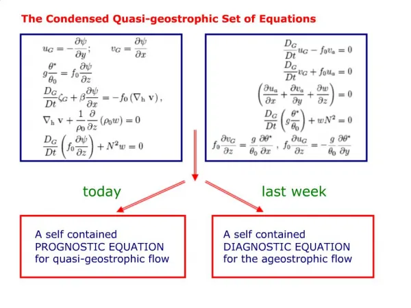
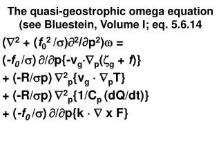
Quasi-geostrophic theory (Continued). John R. Gyakum. The quasi-geostrophic omega equation:. ( s 2 + f 0 2 2 /∂p 2 ) = f 0 / p{v g (1/ f 0 2 + f )} + 2 {v g (- / p)}+ 2 (heating) +friction. The Q-vector form of the quasi-geostrophic omega equation.

Quasi-geostrophic theory (Continued)
E N D
Presentation Transcript
Quasi-geostrophic theory (Continued) John R. Gyakum
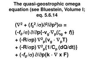
The quasi-geostrophic omega equation: (s2 + f022/∂p2) = f0/p{vg(1/f02 + f)} + 2{vg(- /p)}+ 2(heating) +friction
The Q-vector form of the quasi-geostrophic omega equation (p2 + (f02/)2/∂p2) = (f0/)/p{vgp(1/f02 + f)} + (1/)p2{vgp(- /p)} = -2p Q - (R/p)b(T/x)
Excepting the beffect for adiabatic and frictionless processes: • Where Q vectors converge, there is forcing for ascent • Where Q vectors diverge, there is forcing for descent
5340 m The beta effect: 5400 m Warm Cold Warm -(R/p)b(T/x)<0 X -(R/p)b(T/x)>0
Advantages of the Q-vector approach: • Forcing functions can be evaluated on a constant pressure surface • Forcing functions are “Galilean Invariant” (the functions do not depend on the reference frame in which they are being measured)…although the temperature advection and vorticity advection terms are each not Galilean Invariant, the sum of these two terms is Galilean Invariant • There is not partial cancellation between terms as there typically is with the traditional formulation
Advantages of the Q-vector approach (continued): • The Q-vector forcing function is exact, under the adiabatic, frictionless, and quasi-geostrophic approximation; no terms have been neglected • Q-vectors may be plotted on analyses of height and temperature to obtain a representation of vertical motions and ageostrophic wind
However: • One key disadvantage of the Q-vector approach is that Q-vector divergence is not as physically meaningful as is seen in either horizontal temperature advection or vorticity advection • To remedy this conceptual difficulty, Hoskins and Sanders (1990) have proposed the following analysis:
Q = -(R/p)|T/y|k x(vg/x)where the x, y axes follow respectively, the isotherms, and the opposite of the temperature gradient: isotherms cold y X warm
Q = -(R/p)|T/y|k x(vg/x) Therefore, the Q-vector is oriented 90 degrees clockwise to the geostrophic change vector
To see how this concept works, consider the case of only horizontal thermal advection forcing the quasi-geostrophic vertical motions: Q = -(R/p)|T/y|k x(vg/x) (from Sanders and Hoskins 1990)
Now, consider the case of an equivalent-barotropic atmosphere (heights and isotherms are parallel to one another, in which the only forcing for quasi-geostrophic vertical motions comes from horizontal vorticity advections: Q = -(R/p)|T/y|k x(vg/x) (from Sanders and Hoskins 1990)
(from Sanders and Hoskins 1990): Q = -(R/p)|T/y|k x(vg/x) Q-vectors in a zone of geostrophic frontogenesis: Q-vectors in the entrance region of an upper-level jet
Static stability influence on QG omega • Consider the QG omega equation: (s2 + f022/∂p2) = f0/p{vg(1/f02 + f)} +2{vg(- /p)} + 2(heating)+friction • The static stability parameter s=-T ln/p
Static stability (continued) 1. Weaker static stability produces more vertical motion for a given forcing 2. Especially important examples of this effect occur when cold air flows over relatively warm waters (e.g.; Great Lakes and Gulf Stream) during late fall and winter months 3. The effect is strongest for relatively short wavelength disturbances
Static stability (Continued)1. The ‘effective’ static stability is reduced for saturated conditions, when the lapse rate is referenced to the moist adiabatic, rather than the dry adiabat2. Especially important examples of this effect occur in saturated when cold air flows over relatively warm waters (e.g.; Great Lakes and Gulf Stream) during late fall and winter months3. The effect is strongest for relatively short wavelength disturbances and in warmer temperatures
Static stability • Conditional instability occurs when the environmental lapse rate lies between the moist and dry adiabatic lapse rates: Gd > g > Gm • Potential (or convective) instability occurs when the equivalent potential temperature decreases with elevation (quite possible for such an instability to occur in an inversion or absolutely stable conditions)
Cross-sectional analyses: temperature (degrees C) The shaded zone illustrates the transition zone between the upper troposphere’s weak stratification and the relatively strong stratification of the lower stratosphere (Morgan and Nielsen-Gammon 1998). theta (dashed) and wind speed (solid; m per second) What is the shaded zone? Stay tuned!
References: • Bluestein, H. B., 1992: Synoptic-dynamic meteorology in midlatitudes. Volume I: Principles of kinematics and dynamics. Oxford University Press. 431 pp. • Morgan, M. C., and J. W. Nielsen-Gammon, 1998: Using tropopause maps to diagnose midlatitude weather systems. Mon. Wea. Rev., 126, 2555-2579. • Sanders, F., and B. J. Hoskins, 1990: An easy method for estimation of Q-vectors from weather maps. Wea. and Forecasting, 5, 346-353.