The Quasi-Geostrophic Omega Equation (without friction and diabatic terms)

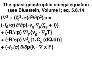
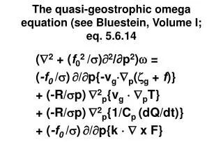
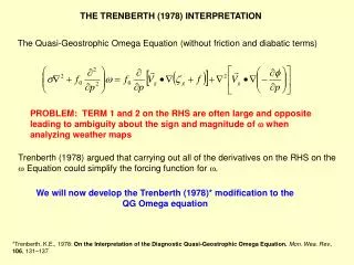
1. THE TRENBERTH (1978) INTERPRETATION The Quasi-Geostrophic Omega Equation (without friction and diabatic terms) PROBLEM: TERM 1 and 2 on the RHS are often large and opposite leading to ambiguity about the sign and magnitude of  when analyzing weather maps Trenberth (1978) argued that carrying out all of the derivatives on the RHS on the  Equation could simplify the forcing function for . We will now develop the Trenberth (1978)* modification to the QG Omega equation *Trenberth, K.E., 1978: On the Interpretation of the Diagnostic Quasi-Geostrophic Omega Equation.Mon. Wea. Rev., 106, 131–137

2. QG OMEGA EQUATION: EXPAND THE ADVECTION TERMS: USE THE EXPRESSIONS FOR THE GEOSTROPHIC WIND AND GEOSTROPHIC VORTICITY: To Get:

3. EXPAND ALL THE DERIVATIVES THEN USE THE JACOBIAN OPERATOR TO SIMPLIFY NOTATION RESULT:

4. Opposite term: opposite sign = same term Same term: opposite sign Deformation Terms in Sutcliff eqn Trenberth: Ignore deformation terms (removes frontogenetic effects) Approximate last term = 2  last term

5. Expand Jacobian terms: This result says that large scale vertical motions can be diagnosed by Examining the advection of absolute vorticity by the thermal wind RECALL SUTCLIFF’S EQUATION SAME INTERPRETATION!!

6. The Geostrophic paradox Confluent geostrophic flow will tighten temperature gradient, leading to an increase in shear via the thermal wind relationship…….. ……but advection of geostrophic momentum by geostrophic wind decreases the vertical shear in the column so…geostrophic flow destroys geostrophic balance!

7. The geostrophic paradox: a mathematical interpretation y momentum equation (QG) Thermodynamic energy equation (QG) For the moment, let’s ignore the ageostrophy (no uag and no ) Let’s look at this equation Take vertical derivative of first equation

8. Expand the derivative: Substitute using the thermal wind relationship: to get: Remember equation in blue box

9. The geostrophic paradox: a mathematical interpretation y momentum equation (QG) Thermodynamic energy equation (QG) For the moment, let’s ignore the ageostrophy (no uag and no ) Now let’s look at this equation Take x derivative of second equation

10. Expand the derivative and use vector notation: Now recall first saved equation: Let’s take these two blue boxed equations and compare them…..

11. thermal wind balance Following the geostrophic wind the magnitude of the temperature gradient and the vertical shear have opposite Tendencies TIGHTENING THE TEMPERATURE GRADIENT WILL REDUCE THE SHEAR!

12. The Geostrophic paradox: RESOLUTION • A separate “ageostrophic • circulation” must exist that • restores geostrophic balance that • simultaneously: • Decreases the magnitude of the horizontal temperature gradient • 2) Increases the vertical shear

13. The Q-Vector interpretation of the Q-G Omega Equation (Hoskins et al. 1978) From consideration of the geostrophic wind, we derived these equations: Let’s denote the term on the RHS: If we start with our original equations, below, y momentum equation (QG) Thermodynamic energy equation (QG) and perform the same operations as before, but with the ageostrophic terms included….

14. We arrive at: With ageostrophic terms Only geostrophic terms Note that the additional terms represent the ageostrophic circulation that works to reestablish geostrophic balance as air accelerates in unbalanced flow.

15. With ageostrophic terms Let’s multiply the bottom equation by -1 and add it to the top equation, recalling that Let’s do the same operations with the x equation of motion and the thermodynamic equation. If we do, we find that:

16. Let’s do the same operations with the x equation of motion and the thermodynamic equation. Where: and:

17. A B Take Substitute continuity equation And use vector notation to get:

18. COMPARE THIS EQUATION WITH THE TRADITIONAL QG  EQUATION! We can write the Q-vector form of the QG  equation as: Where the components of the Q vector are

19. Using the hydrostatic relationship, we can write Q more simply as: or in scalar notation as

20. First note that if the Q vector is convergent Therefore air is rising when the Q vector is convergent

21. Let’s go back to our jet entrance region Q divergence Q convergence Note that there is no in this particular jet The Q vectors capture the sense of the ageostrophic circulation and allow us to see where the rising motion is occurring

22. Resolution of the Geostrophic Paradox Q divergence The Q vectors capture the sense of the ageostrophic circulation and allow us to see where the rising motion is occurring Q convergence Q vectors diagnose a thermally direct circulation Adiabatic cooling of rising warm air Adiabatic warming of sinking cold air Counteracts the tendency of the geostrophic temperature advection in confluent flow Under influence of Coriolis force, horizontal branches tend to increase shear Counteracts the tendency of the geostrophic Momentum advection in the confluent flow

23. A natural coordinate version of the Q vector (Sanders and Hoskins 1990) Consider a zonally oriented confluent entrance region of a jet where Use non-divergence of geostrophic wind or

24. A natural coordinate version of the Q vector (Sanders and Hoskins 1990) Consider a meridionally oriented confluent entrance region of a jet where Use non-divergence of geostrophic wind or

25. A natural coordinate version of the Q vector (Sanders and Hoskins 1990) Using these two expressions, let’s adopt A natural coordinate expression for Q Adopt a coordinate system where is directed along the isotherms is directed normal to the isotherms Q vector oriented perpendicular to the vector change in the geostrophic wind along the isotherms. Magnitude proportional to temperature gradient and inversely proportional to pressure.

26. rising motion sinking motion Simple Application #1 Train of cyclones and anticyclones At center of highs and lows: Black arrows: Gray arrows = Bold arrows = Note also that because of divergence/convergence, train of cyclones and anticyclones propagates east along direction of thermal wind

27. sinking motion rising motion Simple Application #2 Pure deformation flow with a temperature gradient Along axis of dilitation Black arrows: Gray arrows = Bold arrows = Increases toward east

28. Simple Application #3 Homogeneous warm advection No variation in Black arrows: Gray arrows = Bold arrows = along an isotherm No heterogeneity in the warm advection field = No rising motion!

29. Note that the Q vector form of the QG -equation contains the deformation terms (unlike the Sutcliff and Trenberth forms) And combines the vorticity and thermal advection terms into a single diagnostic (unlike the traditional QG -equation) Deformation term contribution to  Sutcliff/Trenberth approximation

30. The along and across-isentrope components of the Q vector Begin with the hydrostatic equation in potential temperature form where: (which is constant on an isobaric surface) And the definition of the Q vector: Substituting: This expression is equivalent to:

31. The Q-vector describes the rate of change of the potential temperature along The direction of the geostrophic flow Let’s consider separately the components of Q along and across the isentropes

32. Is parallel to and can only affect changes in the magnitude of Is perpendicular to and can only affect changes in the direction of

33. Returning to QG  equation Components of vertical motion can be distributed in couplets across (transverse to) the thermal wind (mean isotherms) and along (shearwise) the thermal wind. We will see later that the transverse component of Q is related to the dynamics of frontal zones.