Download
1 / 16
160 likes | 502 Vues
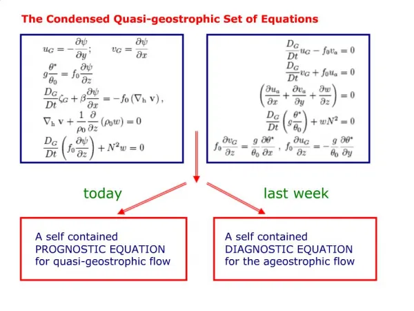
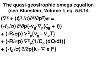
Quasi-geostrophic omega analyses. John Gyakum ATOC-541 January 4, 2006. Outline. The QG omega equation and its physical interpretation. The quasi-geostrophic omega equation:. ( s 2 + f 0 2 2 /∂p 2 ) = f 0 / p{v g (1/ f 0 2 + f )}

E N D
Quasi-geostrophic omega analyses John Gyakum ATOC-541 January 4, 2006
Outline • The QG omega equation and its physical interpretation
The quasi-geostrophic omega equation: (s2 + f022/∂p2) = f0/p{vg(1/f02 + f)} + 2{vg(- /p)}+ 2(heating) +friction
Before considering the physical effects of the quasi-geostrophic forcing, consider the thermal vorticity: Thermal= geostrophic Top- geostrophic Bottom = (g/f) times (2zTop - 2zBottom) = (g/f) times (2h) Where h = zTop - zBottom = thickness
Therefore, the thermal vorticity is the algebraic difference between the top and bottom geostrophic vorticity A cold pool of air is also a thermal vorticity maximum Top pressure Top Pressure (low) cold cold Bottom Pressure (high) Bottom Pressure
Therefore, a cold trough is a thermal vorticity maximum Consider the ‘vorticity advection’ forcing for The quasi-geostrophic vorticity equation: (s2 + f022/∂p2) = f0/p{vg(1/f02 + f)} + ...
An upward increase in cyclonic vorticity advection(or an upward decrease in anticyclonic vorticity advection)produces an increase in cyclonic thermal vorticity, which cools the column locally How does this cooling occur? Local change in temperature= Horizontal temperature advection + vertical motions + diabatic changes
Thus, the only means of cooling the column is throughascent in a hydrostatically stable atmosphere 1. The thickness is decreasing 2. The heights are falling at all levels, but more so aloft 3. Convergence is responsible for the vorticity increase below 4. ‘PVA’ overwhelms the effects of divergence aloft top z/t -/t V bottom - 0 + - 0 +
Now consider the effect of warm advection in the quasi-geostrophic omega equation (s2 + f022/∂p2) = + 2{vg(- /p)}+... Warming produces an increase in thickness and a warm ridge locally; Therefore, Thermal/t < 0
1. The thickness is increasing 2. Divergence is responsible for all Vorticity changes…because of mass Continuity, the vertical integral of Vorticity change must be zero And… geostrophic upper/t < geostrophic lower/t So,…how is this done??? The vorticity changes must occur Only through divergence/ Convergence, since there is no Vorticity advection. Therefore, we must have the Divergence structure seen here: top V z/t -/t bottom - 0 +
Note that the diabatic effects of heating have the same mathematical structure as for the horizontal temperature advection effect: (s2 + f022/∂p2) = + 2{vg(- /p)}+ 2(heating)+...
1. The thickness is increasing 2. Divergence is responsible for all Vorticity changes…because of mass Continuity, the vertical integral of Vorticity change must be zero Therefore: And… geostrophic upper/t < geostrophic lower/t top The vorticity changes must occur Only through divergence/ Convergence, since there is no Vorticity advection. Therefore, we must have the Divergence structure seen here: V z/t -/t bottom
Diabatic heating effects • Regions of surface sensible heat flux (particularly strong in cold-air outbreaks over relatively warm waters; e. g. Great Lakes in late autumn, early winter; cold outbreaks over the Gulf Stream current of the North Atlantic) • Regions of latent heating (stratiform and moist convection)
Current synoptic conditions (1200 UTC, 4 January 2006; Eta model SLP; 1000-500 hPa thickness)
The 300-hPa heights and isotachs for 1200 UTC, 4 January 2006
Reference: • Bluestein, H. B., 1992: Synoptic-dynamic meteorology in midlatitudes. Volume I: Principles of kinematics and dynamics. Oxford University Press. 431 pp.