Quasi-Geostrophic (QG) Theory

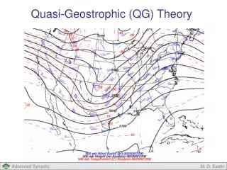
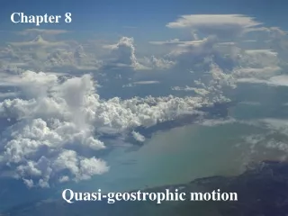
1. Quasi-Geostrophic (QG) Theory M. D. Eastin

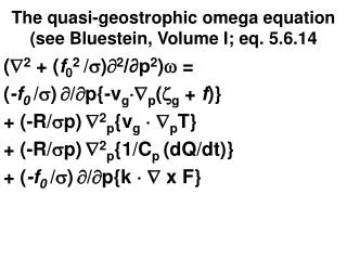
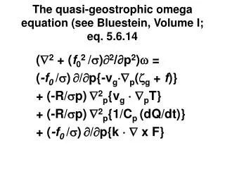
2. Quasi-Geostrophic (QG) Theory • QG Theory • Basic Idea • Approximations and Validity • QG Equations / Reference • QG Analysis • Basic Idea • Estimating Vertical Motion • QG Omega Equation: Basic Form • QG Omega Equation: Relation to Jet Streaks • QG Omega Equation: Q-vector Form • Estimating System Evolution • QG Height Tendency Equation • Diabatic and Orographic Processes • Evolution of Low-level Cyclones • Evolution of Upper-level Troughs M. D. Eastin

3. QG Theory: Basic Idea • Forecast Needs: • The public desires information regarding temperature, humidity, precipitation, • and wind speed and direction up to 7 days in advance across the entire country • Such information is largely a function of the evolving synoptic weather patterns • (i.e., surface pressure systems, fronts, and jet streams) • Four Forecast Methods: • Conceptual Models: Based on numerous observations from past events • Generalization of the synoptic patterns • Polar-Front theory • Kinematic Approach: Analyze current observations of wind, temperature, and moisture fields • Assume clouds and precipitation occur when there is upward motion • and an adequate supply of moisture • QG theory • Numerical models: Based on integration of the primitive equations forward in time • Require dense observations, and accurate physical parameterizations • User must compensate for erroneous initial conditions and model errors • Statistical models: Use observations or numerical model output to infer the likelihood of • of certain meteorological events M. D. Eastin

4. QG Theory: Basic Idea • What will QG Theory do for us? • It reveals how hydrostatic balance and geostrophic balance constrain • and simplify atmospheric motions, but in a realistic manner • It provides a simple framework within which we can understand and • diagnose the vertical motion and evolution of three-dimensional • synoptic-scale weather systems • It helps us to understand how the mass fields (via horizontal temperature • advection) and the momentum fields (via horizontal vorticity advection) • interact to create vertical circulations that result in realistic synoptic- • scale weather patterns • It offers physical insight into the forcing of vertical motion and • cloud/precipitation patterns associated with mid-latitude cyclones M. D. Eastin

5. QG Theory: Approximations and Validity • What do we already know? • The primitive equations are quite complicated • For mid-latitude synoptic-scale motions the horizontal winds are nearly geostrophic • (i.e., they are quasi-geostrophic) above the surface • We can use this fact to further simplify the equations, and still maintain accuracy M. D. Eastin

6. QG Theory: Approximations and Validity • Start with: • Primitive equations in isobaric coordinates (to simplify the dynamics) • Hydrostatic Balance (valid for synoptic-scale flow) • Frictionless Flow (neglect boundary-layer and orographic processes) Zonal Momentum Meridional Momentum Hydrostatic Approximation Mass Continuity Thermodynamic Equation of State M. D. Eastin

7. QG Theory: Approximations and Validity • Split the total horizontal velocity into geostrophicand ageostrophic components • (ug, vg) → geostrophic → portion of the total wind in geostrophic balance • (uag, vag) → ageostrophic → portion of the total wind NOT in geostrophic balance • Recall the horizontal equations of motion (isobaric coordinates): • where and M. D. Eastin

8. QG Theory: Approximations and Validity • Perform a scale analysis of the acceleration and Coriolis terms (construct ratios): • For typical mid-latitude synoptic-scale systems: • Our scale analysis implies a smallRossby Number (Ro): • where M. D. Eastin

9. QG Theory: Approximations and Validity • Thus, we can assume: • →→ →→ • Since by definition We can also assume: • (geostrophic balance) • →→ →→ • If the ageostrophic component of the wind is small then, we can assume: • where: • Note: This does NOT mean the ageostrophic components are unimportant M. D. Eastin

10. QG Theory: Approximations and Validity • Thus, the primary assumption (or simplification) of QG theory is: • Ro is small → (a) ageostrophic flow is assumed to be < 10% of geostrophic flow • (b) horizontal advection is accomplished by only the geostrophic flow • (c) no vertical advection in the total derivative • What do our “new” equations of motion look like? • What do we do with the Coriolis accelerations? M. D. Eastin

11. QG Theory: Approximations and Validity • We can make anotherassumption about the Coriolis parameter (f)that will ultimately • simplify our full system of equations: • Approximate the Coriolis parameter with a Taylor Series expansion: • →→ • where: is the Coriolis parameter at a constant reference latitude • is the constant meridional gradient in the Coriolis parameter • If we perform a scale analysis on the two terms, we find: • and we can re-write our geostrophic balance equations as: →→ →→ M. D. Eastin

12. QG Theory: Equations of Motion • If we now combine (a) our expanded Coriolis parameter with (b) our new geostrophic • balance equations, and apply the small Rossby number assumption, we obtain • the “final” QG momentum equations: • These are (2.14) and (2.15) • in the Lackmann text Physical Interpretation:(1) Accelerations in the geostrophic flow result entirely from ageostrophic flow associated with the Coriolis force (2) The Coriolis “torque” acting at right angles to the ageostrophic wind lead to accelerations in the geostrophic wind components perpendicular to the ageostrophic motions M. D. Eastin

13. QG Equations: Continuity Equation • Startwith the primitive form of the mass continuity equation in isobaric coordinates: • Substitute in: and then using: • One can easily show that the geostrophic flow is non-divergent, or • Thus, the QG continuity is: • This is (2.17) in the Lackmann text • Physical Interpretation: The vertical velocity (ω) depends only on the ageostrophic • components of the flow M. D. Eastin

14. QG Equations: Thermodynamic Equation • Start with the primitive form of the thermodynamic equation in isobaric coordinates: • We can combine the two terms containing vertical motion (ω) and apply • the primary assumption of QG theory, such that • This is (2.18) in the where: • Lackmann text • Finally, (a) neglect diabatic heating (J) [for now…we will return to this later] • (b) assume static stability (σ) is only a function of pressure • Physical Interpretation: (a) geostrophic flow is adiabatic (no latent heating) • (b) horizontally-uniform static stability (CAPE is the same) M. D. Eastin

15. QG Equations: Vorticity Equation • Start with the “final” QG momentum equations: • Zonal Momentum • Meridional Momentum • Take of the meridional equation and subtract the of the zonal equation: • Then, after some algebra, invoking non-divergent geostrophic flow, and substituting • the QG continuity equation, we get: • where: • Physical Interpretation: The total rate change of geostrophic relative vorticity is • a function of (a) the geostrophic advection of planetary • vorticity and (b) vortex stretching M. D. Eastin

16. QG Equations: Vorticity Equation • Let’s look at the physical interpretations in greater detail: • Term 1Term 2Term 3Term 4 • Term 1: Local time rate of change in geostrophic relative vorticity • Term 2: Horizontal advection of geostrophic relative vorticity by the geostrophic flow • Positive vorticity advection (PVA) will increase the local vorticity • Negative vorticity advection (NVA) will decrease the local vorticity • Term 3: Meridional advection of planetary vorticity by the geostrophic flow • Beta (β) is always positive • Positive (or northward) meridional flow will decrease the local vorticity • Negative (or southward) meridional flow will increase the local vorticity • Term 4: Addition (subtraction) of vorticity due to stretching (shrinking) of the column • An increase in the vertical motion with height will increase the local vorticity A decrease in vertical motion with height will decrease the local vorticity M. D. Eastin

17. QG Equations: Reference Summary of the QG Equations: Decomposition of Total Winds Geostrophic Balance Coriolis Approximation Zonal Momentum Equation Meridional Momentum Equation Continuity Equation Geostrophic Non-divergence Adiabatic Thermodynamic Equation Static Stability Vorticity Equation Relative Vorticity M. D. Eastin

18. QG Theory: Summary • QG Theory – Underlying (Limiting) Assumptions • Small Rossby Number (advection by only the geostrophic flow) • Hydrostatic Balance • Frictionless flow • No orographic effects ** • No diabatic heating or cooling ** • Horizontally uniform static stability **We will discuss how to compensate for these two limitations as we progress through each topic M. D. Eastin

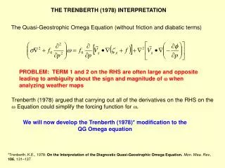
19. References Bluestein, H. B, 1993: Synoptic-Dynamic Meteorology in Midlatitudes. Volume I: Principles of Kinematics and Dynamics. Oxford University Press, New York, 431 pp. Bluestein, H. B, 1993: Synoptic-Dynamic Meteorology in Midlatitudes. Volume II: Observations and Theory of Weather Systems. Oxford University Press, New York, 594 pp. Charney, J. G., B. Gilchrist, and F. G. Shuman, 1956: The prediction of general quasi-geostrophic motions. J. Meteor., 13, 489-499. Hoskins, B. J., I. Draghici, and H. C. Davis, 1978: A new look at the ω–equation. Quart. J. Roy. Meteor. Soc., 104, 31-38. Hoskins, B. J., and M. A. Pedder, 1980: The diagnosis of middle latitude synoptic development. Quart. J. Roy. Meteor. Soc., 104, 31-38. Lackmann, G., 2011: Mid-latitude Synoptic Meteorology – Dynamics, Analysis and Forecasting, AMS, 343 pp. Trenberth, K. E., 1978: On the interpretation of the diagnostic quasi-geostrophic omega equation. Mon. Wea. Rev., 106, 131-137. M. D. Eastin