DAY 3

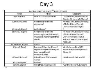
1. DAY 3 14 Jan 2014

2. Today is • January 14, 2014 • January 13, 2013

3. Recap • Organizing Data • Qualitative & Quantitative Data • Frequency distribution & relative frequency distribution • Single-value grouping, Limit grouping, Cut point grouping • Histogram, Dotplots, Stem-and-leaf diagrams

4. Objective of the day: • Distribution shapes • Descriptive Measures => Central Measures => Mean, Median, Mode. • Measures of Variations => Standard Deviation

5. Section 2.4 Distribution Shapes

6. Definition 2.10 Distribution of a Data Set The distribution of a data set is a table, graph, or formula that provides the values of the observations and how often they occur.

7. Relative-frequency histogram and approximating smooth curve for the distribution of heights

8. Common distribution shapes

9. Example: Relative-frequency histogram for household size Identify the shape of the distribution.

10. Example: Relative-frequency histogram for household size Identify the shape of the distribution.

14. Definition 2.12 Population and Sample Distributions; Distribution of a Variable The distribution of population data is called the population distribution, or the distribution of the variable. The distribution of sample data is called a sample distribution.

15. Population distribution and six sample distributions for household size

16. Key Facts: Population and Sample Distributions For a simple random sample, the sample distribution approximates the population distribution (i.e., the distribution of the variable under consideration). The larger the sample size, the better the approximation tends to be.

17. Chapter 3 Descriptive Measures

18. Descriptive Measures Number that describe data set.

19. Section 3.1 Measures of Center

20. Measure of Center Descriptive measures that indicates where the center or most typical value of data set lies are called measure of central tendency or measures of center. Three most important measures of center: • Mean • Median • Mode

22. Definition 3.1 Mean of a Data Set The mean of a data set is the sum of the observations divided by the number of observations. mean= sum of the observations / the number of observations.

23. Example: Data Set II Data Set I

24. Example: Data Set II Data Set I Meansin Data Set I and Data Set II

25. Definition 3.2 Median of a Data Set Arrange the data in increasing order. • If the number of observations is odd, then the median is the observation exactly in the middle of the ordered list. • If the number of observations is even, then the median is the mean of the two middle observations in the ordered list. In both cases, if we let n denote the number of observations, then the median is at position (n + 1) / 2 in the ordered list.

26. Definition 3.3 Mode of a Data Set Find the frequency of each value in the data set. • If no value occurs more than once, then the data set has no mode. • Otherwise, any value that occurs with the greatest frequency is a mode of the data set.

29. Example: Data Set I Median in Data Set I Data Set I 300 300 300 300 300 300 400 400 450 450 800 940 1050 Median is at the position (n+1)/2 = (13+1)/2 = 7 Median = ?

30. Example: Data Set I Median in Data Set I Data Set I 300 300 300 300 300 300 400 400 450 450 800 940 1050 Median is at the position (n+1)/2 = (13+1)/2 = 7 Median = 400

31. Example: Data Set I Mode in Data Set I Data Set I 300 300 300 300 300 300 400 400 450 450 800 940 1050 Mode = ?

32. Example: Data Set I Mode in Data Set I Data Set I 300 300 300 300 300 300 400 400 450 450 800 940 1050 Mode = 300

33. Example: Data Set II Data Set I Mean, Median, and Mode in Data Set I and Data Set II

34. Definition 3.4

35. ƒ COMPARISON OF MEAN, MEDIAN, MODE: 1. Note that the mean is pulled in the direction of the skewness, i.e. in the direction of the extreme observation. The mean is sensitive to extreme observations (very large or very small in comparison to the rest of the data). The mean is not a resistant measure of center. 2. The median is not pulled into the direction of the most extreme observations. The median is not sensitive to extremes, i.e. the median is a resistant measure of center. 3. When the data is skewed, therefore, the median is the preferred measure of center. 4. The mode may not be near the center and, thus not useful as a measure of center.

36. Relative positions of the mean and median for (a) right-skewed, (b) symmetric, and (c) left-skewed distributions

40. Section 3.2 Measures of Variation

41. Example: Five starting players on two basketball teams

42. Example: Shortest and tallest starting players on the teams

43. Definition 3.5 Range of a Data Set The range of a data set is given by the formula Range = Max – Min, where Max and Min denote the maximum and minimum observations, respectively.

44. ∑ 10 10 ∑ N = 1+2+3+4+5+6+7+8+9+10 ∑ N = ? N = 1 N = 1

45. Definition 3.6

46. Example: Five starting players on basketball Team I.

47. Example: Five starting players on basketball Team I

48. Example: Five starting players on basketball Team I

49. Example: Five starting players on basketball Team II

50. Example: Five starting players on basketball Team 1.