Exploring Symmetry Detection in Constraint Satisfaction Problems and Its Database Applications

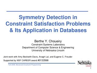
1. Symmetry Detection in Constraint Satisfaction Problems & Its Application in Databases Berthe Y. Choueiry Constraint Systems Laboratory Department of Computer Science & Engineering University of Nebraska-Lincoln Joint work with Amy Beckwith-Davis, Anagh Lal, and Eugene C. Freuder Supported by NSF CAREER award #0133568

2. Outline • Definitions • CSP • Interchangeability • Bundling • Bundling in CSPs • Bundling for join query computation • Conclusions

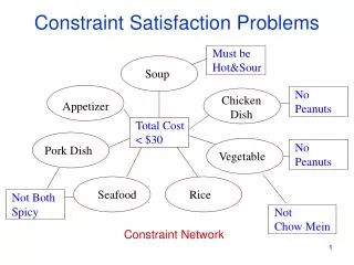
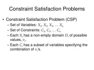
3. V1 V2 {c, d, e, f} {d} V4 V3 {a, b, d} {a, b, c} Constraint Satisfaction Problem (CSP) • GivenP = (V, D, C) • V : set of variables • D : set of their domains • C : set of constraints (relations) restricting the acceptable combination of values for variables • Solution is a consistent assignment of values to variables • Query: find 1 solution, all solutions, etc. • Examples: SAT, scheduling, product configuration • NP-Complete in general

4. Solution V1 d V2  e V3  a V4  c V1 d V1 V2 { c, d, e, f} {d} V2 {c,d,e,f} V3 V4 {a,b,d} V3 {a, b, d} {a, b, c} V4 {a,b,c} Backtrack search S • DFS + backtracking (linear space) • Variable being instantiated: current variable • Un-instantiated variables: futurevariables • Instantiated variables: pastvariables • + Constraint propagation • Backtrack search with forward checking (FC) d V1 V2 c e f d V3

5. V1 V2 { c, d, e, f} {d} In every solution V1 d V1 d V1  V2  c V2  c V4 V2  {d, e, f} V3 {a, b, d} {a, b, c} V3 a V3 b V3  V4 b V4 a V4  Interchangeability [Freuder, 91] • Captures the idea of symmetry between solutions • Functional interchangeability • Any mapping between two solutions • Including permutation of values across variables, equivalent to graph isomorphism • Full interchangeability (FI) • Restricted to values of a single variable • Also, likely intractable

6. Value interchangeability [Freuder, 91] • Full Interchangeability (FI): • d, e, finterchangeable for V2 in any solution • Neighborhood Interchangeability (NI): • Considers only the neighborhood of the variable • Finds e, f but misses d • Efficiently approximates FI • Discrimination tree DT(V2) {c, d, e, f } {d} V1 V2 {a, b, d} {a, b, c} V3 V4

7. Outline • Definitions • Bundling in CSPs • Static bundling • Dynamic bundling • Dynamic bundling for non-binary CSPs • Bundling for join query computation • Conclusions

8. V1 d V2  {e,f} V3  a V1 V2 { c, d, e, f } {d} S V1 d V4 V3 V2 {a, b, d} {a, b, c} c e, f d Bundling: using NI in search V1 { c, d, e, f } V2 { c, d, e, f } { d, c, e, f } V4  {b,c} V3 Static bundling V4 • Static bundling [Haselböck, 93] • Before search: compute & store NI sets • During search: • Future variables: remove bundle of equivalent values • Current variable: assign a bundle of equivalent values • Advantages • Reduces search space • Creates bundled solutions

9. V1 V2 { c, d, e, f } {d} S S V1 V1 d d V4 V3 V2 V2 {a, b, d} {a, b, c} c e, f d c d, e, f Dynamic bundling (DynBndl) [2001] • Dynamically identifies NI • Using discrimination tree for forward checking: • is never less efficient than BT & static bundling <V3,a> <V3,b> <V4,a> <V3,d> <V4,a> <V4,b> <V4,c> <V4,b> V2,{c} V2,{d,e,f} Static bundling Dynamic bundling

10. V {1, 2, 3} Constraint V3 {1, 2, 3, 4, 5, 6} Variable C2 {1, 2, 3} V2 C1 V4 {1, 2, 3} C3 {1, 2, 3} V1 C4 Non-binary CSPs • Scope(Cx): the set of variables involved in Cx • Arity(Cx): size of scope Computing NI for non-binary CSPs is not a trivial extension from binary CSPs

11. C2 V {1, 2, 3, 4, 5, 6} V3 C1 V2 V4 C3 V1 C4 {1, 2} {3, 4} {5} {6} NI for non-binary CSPs [2003,2005] • Building an nb-DT for each constraint • Determines the NI sets of variable given constraint • Intersecting partitions from nb-DTs • Yields NI sets of V (partition of DV) • Processing paths in nb-DTs • Gives, for free, updates necessary for forward checking Root Root {5} {1, 2} {5, 6} {3, 4} {3, 4} {6} {1, 2} nb-DT(V, C1) nb-DT(V, C2)

12. V1 d V1 d V2  {e,f} V2  e V3  a V3  a V4  {b,c} V4  c Robust solutions Single Solution Static bundling Dynamic bundling • Solution bundle • Cartesian product of domain bundles • Compact representation • Robust solutions • Dynamic bundling finds larger bundles V1 d V2  {d,e,f} V3  a V4  {b,c}

13. DynBndl: worth the effort? • Finds larger bundles • Enables forward checking at no extra cost • Does not cost more than BT or static bundling • Cost model: • # nodes visited by search • # constraint checks made • Theoretical guarantee holds • for finding all solutions • under same variable ordering • Finding first solution ? • Experiments uncover an unexpected benefit

14. V {3, 4} {1, 2} V3 V {1, 2, 3} C2 {1, 2, 3, 4, 5, 6} V1 {1, 3} {1} V2 C1 {1, 2, 3} V4 {1, 2, 3} {1} C3 {3} V2 V1 C4 {1, 2, 3} V3 {2} {1} V4 Bundling of no-goods… • … is particularly effective No-good bundle Solution bundle

15. Mostly un-solvable instances Mostly solvable instances Cost of solving Order parameter Critical value Experimental set-up • CSP parameters: • n: number of variables {20,30} • a: domain size {10,15} • t: constraint tightness [25%, 75%] • CR: constraint ratio (arity: 2, 3, 4) • 1,000 instances per tightness value • Phase transition • Performance measures • Nodes visited (NV) • Constraint checks (CC) • CPU time • First Bundle Size (FBS)

16. Empirical evaluations • DynBndl versus FC (BT + forward checking) • Randomly generated problems, Model B • Experiments • Effect of varying tightness • In the phase-transition region • Effect of varying domain size • Effect of varying constraint ratio (CR) • ANOVA to statistically compare performance of DynBndl and FC with varying t • t-distribution for confidence intervals

17. Analysis: Varying tightness • Low tightness • Large FBS • 33 at t=0.35 • 2254 (Dataset #13, t=0.35) • Small additional cost • Phase transition • Multiple solutions present • Maximum no-good bundling causes max savings in CPU time, NV, & CC • High tightness • Problems mostly unsolvable • Overhead of bundling minimal FC 20 n=20 t FBS 0.350 33.44 a=15 18 Time [sec] DynBndl 0.400 10.91 CR=CR3 16 #NV, hundreds 0.425 7.13 0.437 6.38 14 0.450 5.62 12 0.462 2.37 FC 0.4750.66 10 0.500 0.03 NV 8 0.550 0.00 6 DynBndl 4 2 CPU time 0 0.325 0.35 0.375 0.4 0.425 0.45 0.475 0.5 0.525 0.55 0.575 0.6 Tightness

18. Analysis: Varying domain size • Increasing a in phase-transition • FBS increases: More chances for symmetry • CPU time decreases: more bundling of no-goods Increasing a (n=30) Because the benefits of DynBndl increase with increasing domain size, DynBndl is particularly interesting for database applications where large domains are typical

19. Outline • Definitions • Bundling in CSPs • Bundling for join query computation • Idea • A CSP model for the query join • Sorting-based bundling algorithm • Dynamic-bundling-based join algorithm • Conclusions

20. The join query Join query • SELECT R2.A,R2.B,R2.C • FROM R1,R2 • WHERE R1.A=R2.A • AND R1.B=R2.B • AND R1.C=R2.C (compacted) R1 R2 Result: 10 tuples in 3 nested tuples A B C {1, 5} {12, 13, 14} {23} {2, 4} {10} {25} {6} {13, 14} {27}

21. Databases & CSPs • Same computational problems, different cost models • Databases: minimize # I/O operations • CSP community: # CPU operations • Challenges for using CSP techniques in DB • Use of lighter data structures to minimize memory usage • Fit in the iterator model of database engines

22. R1.A R1.B R1.C R2 R1 R2.C R2.A R2.B Modeling join query as a CSP • Attributes of relations  CSP variables • Attribute values  variable domains • Relations  relational constraints • Join conditions  join-condition constraints • SELECT R1.A,R1.B,R1.C • FROM R1,R2 • WHERE R1.A=R2.A • AND R1.B=R2.B • AND R1.C=R2.C

23. Join operator • R1 xyR2 • Most expensive operator in terms of I/O •  is “=”  Equi-Join • x is same as y  Natural Join • Join algorithms • Nested Loop • Sorting-based • Sort-Merge, Progressive Merge-Join (PMJ) • Partitions relations by sorting, minimizes # scans of relations • Hashing-based

24. R1.A R1.B R1.C R2 R1 R2.C R2.A R2.B Join query • R1 xyR2 • Most expensive operator in terms of I/O •  is “=”  Equi-Join • x is same as y  Natural Join • CSP model • Attributes of relations  CSP variables • Attribute values  variable domains • Relations  relational constraints • Join conditions  join-condition constraints • SELECT R1.A,R1.B,R1.C • FROM R1,R2 • WHERE R1.A=R2.A • AND R1.B=R2.B • AND R1.C=R2.C

25. Progressive Merge Join • PMJ: a sort-merge algorithm [Dittrich et al. 03] • Two phases • Sorting: sorts sub-sets of relations & • Merging phase: merges sorted sub-sets • PMJ produces early results • We use the framework of the PMJ

26. New join algorithm • Sorting & merging phases • Load sub-sets of relations in memory • Compute in-memory join using dynamic bundling • Uses sorting-based bundling (shown next) • Computes join of in-memory relations using dynamically computed bundles

27. Sorting-based bundling R1.A • Heuristic for variable ordering Place variables linked by join conditions as close to each other as possible R2.A R1 R1.B R2.B R2 R1.C R2.C • Sort relations using above ordering • Next: Compute bundles of variable ahead in variable ordering (R1.A)

28. Computing a bundle of R1.A • Partition of a constraint • Tuples of the relation having the same value of R1.A • Compare projected tuples of first partition with those of another partition • Compare with every other partition to get complete bundle R1 A B C 1 12 23 Partition 1 13 23 1 14 23 Unequal partitions 2 10 25 Symmetric partitions 5 12 23 5 13 23 5 14 23 Bundle {1, 5}

29. Finding the valid bundle Common {1, 5} • Compute a bundle for the attribute • Check bundle validity with future constraints • If no common value ‘backtrack’  Assign variable with the surviving values in the bundle {1, 5, x} {1, 5, y, z}

30. Experiments • XXL library for implementation & evaluation • Data sets • Random: 2 relations R1, R2 with same schema as example • Each relation: 10,000 tuples • Memory size: 4,000 tuples • Page size 200 tuples • Real-world problem: 3 relations, 4 attributes • Compaction rate achieved • Random problem: 1.48 • Savings even with (very) preliminary implementation • Real-world problem: 2.26 (69 tuples in 32 nested tuples)

31. Outline • Definitions • Bundling in CSPs • Bundling for join query computation • Conclusions • Summary • Future research

32. Summary • Dynamic bundling in finite CSPs • Binary and non-binary constraints • Produces multiple robust solutions • Significantly reduces cost of search at phase transition • Application to join-query computation Constraint Processing inspires innovative solutions to fundamental difficult problems in Databases

33. Future research • CSPs • Only scratched the surface: • interchangeability + decomposition [ECAI 1996], • partial interchangeability [AAAI 1998], • tractable structures • Databases • Investigate benefit of bundling • Sampling operator • Main-memory databases • Automatic categorization of query results • Constraint databases • Design bundling mechanisms for gap & linear constraints over intervals (spatial databases)