CHAPTER 3 Measurement Systems with Electrical Signals
220 likes | 470 Vues
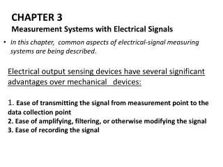
CHAPTER 3 Measurement Systems with Electrical Signals. In this chapter, common aspects of electrical-signal measuring systems are being described. Electrical output sensing devices have several significant advantages over mechanical devices:

CHAPTER 3 Measurement Systems with Electrical Signals
E N D
Presentation Transcript
CHAPTER 3 Measurement Systems with Electrical Signals • In this chapter, common aspects of electrical-signal measuring systems are being described. Electrical output sensing devices have several significant advantages over mechanical devices: 1. Ease of transmitting the signal from measurement point to the data collection point 2. Ease of amplifying, filtering, or otherwise modifying the signal 3. Ease of recording the signal
Stages in electrical signal measuring system. Electrical output transducers are available for almost any measurement. A partial list includes transducers to measure displacement, linear velocity, angular velocity, acceleration, force, pressure, temperature, heat flux, neutron flux, humidity, fluid flow rate, light intensity, chemical characteristics, and chemical composition. sensor and transducer often used interchangeably, There are other words used to name transducers for particular applications-the terms gage,cell,pickup,andtransmitter being common.
SIGNAL CONDITIONERS • There are many possible functions of the signal-conditioning stage. The following are the most common: • Amplification • Attenuation • Filtering (highpass, Iowpass, bandpass, or bandstop) • Differentiation • Integration • Linearization • Combining a measured signal with a reference signal • Converting a resistance to a voltage signal • Converting a current signal to a voltage signal • Converting a voltage signal to a current signal • Converting a frequency signal to a voltage signal More than one signal-conditioning function, such as amplification and filtering, can be performed on a signal.
General Characteristics of Signal Amplification • Many transducers produce signals with low voltages • Signals in the millivolt range are common, and in some cases, signals are in the microvolt range. • It is difficult to transmit such signals over wires of great length, and many processing systems require input voltages on the order of 1 to 10 V. • The amplitude of such signals can be increased using a • device called an amplifier, shown as a block diagram in Fig. The degree of amplification is specified by a parameter called the gain, G: Generic voltage amplifier.
Gain is more commonly stated using a logarithmic scale, and the result is expressed in decibels (dB). For voltage gain, this takes the form Using this formula, an amplifier with G of 10 would have a decibel gain, Gdb, of 20 dB, and an amplifier with a G of 1000 would have a decibel gain of 60. The range of frequencies with close to constant gain is known as the bandwidth. The upper and lower frequencies defining the bandwidth, called the corner or cutoff frequencies,
An amplifier with a narrow bandwidth will change the shape of an input time varying signal by an effect known as frequency distortion. Although the gain of an amplifier will be relatively constant over the bandwidth, another characteristic of the output signal, the phase angle, may change significantly.
The voltage input signal to the amplifier: The outputsignal will be:
The shape of the signal is changed dramatically and shows significant phase distortion'
Another important characteristic of amplifiers is known as common-mode rejection ratio (CMRR). When the same voltage (relative to ground) is applied to the two input terminals, the input is known as a common-mode voltage . Instrumentation amplifier will produce an output in response to differential-mode voltages but will produce no output in response to common- mode voltages. The measure of the relative response to differential- and common mode voltages is described by common-mode rejection ratio, defined by Gdifis the gain for a differential-mode voltage Gcmis the gain for a common-mode voltage High-quality amplifiers often have a CMRR in excess of 100 dB.
Input-loading and output loading are potential problems that can occur when Using an amplifier (and when using many other signal-conditioning devices)'
CHAPTER 3 Continued… Measurement Systems with Electrical Signals • displacement, • linear velocity, • Angular • velocity, • acceleration, • force, • pressure, • temperature, • heat flux, • humidity, • fluid flow rate, • light intensity, • Chemical Characteristic • chemical composition. • Amplification • Attenuation • Filtering (highpass,Iowpass,bandpass, or bandstop) • Differentiation • Integration • Linearization • Converting a resistance to a voltage signal • Converting a current signal to a voltage signal • gage, • cell, • pickup, • Transmitter • Converts physical changes to electrical pulses
Amplifiers Using Operational Amplifiers • Practical signal amplifiers can be constructed using a common, low-cost. Integrated circuit • component called an operational amplifier, or simply an op-amp. An op-amp is represented schematically by a triangular symbol as shown in figure below. • The input voltages (Vn, Vp) are applied to two input terminals (labeled + and -), and • the output voltage (Vo) appears through a single output terminal. • There are two power supply terminals, labeled V+ and V-. Figure 3.10
The op-amp gain is given by small g to distinguish it from G, the gain of amplifier circuits using the op-amp as a component. The output of the op-amp in the open-loop configuration shown in Figure 3.10 is given by
Analyzing the circuit, the current through resistor The current flow from point B into the op-amp negative terminal will be small due to the high op-amp input impedance and will be neglected.
Above fc, the gain starts to decrease, or roll off, and this roll-off occurs at a rate of 6 dB per octave. “octave” is a doubling of the frequency…
This roll off in gain at high frequencies is an inherent characteristic of op-amps. The cutoff frequency, fc, depends on the low-frequency gain of the amplifier-the higher the gain, the lower is fc . This low-frequency gain-cutoff frequency relationship is described by a parameter called the gain-bandwidth product (GBP). For most op-amp- based amplifiers, the product of the low-frequency gain and the bandwidth is a constant. Since the lower frequency limit of the bandwidth is zero, the upper cutoff frequency can be evaluated from Although the gain is constant over the bandwidth, the phase angle between the input and the output, @, shows a strong variation with frequency. For the non-inverting amplifier in Figure 3.11, the phase-angle variation with frequency is given by