Download
1 / 40
400 likes | 438 Vues
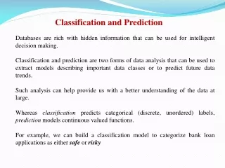
This text covers the basics of classification in predictive methods, including applications like credit approval, medical diagnosis, and fraud detection. It delves into supervised vs. unsupervised learning, classification terminology, model building, validation, and application, emphasizing the importance of accuracy and model comparison.

E N D
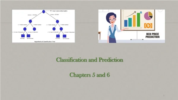
Classification and Prediction Chapters 5 and 6
What is Classification? • A predictive method • Mapping instances onto a predefined set of classes • Model used to classify new data • Some Applications • Credit approval – high vs low risk • Target marketing – loyal vs other customers • Medical diagnosis – cancerous vs benign cells • Fraud – genuine vs fraudulent transactions
5 2.5 25 53 2.5 3 Example 1 Class B Examples A or B? Class A Examples 4 4 8 1.5 5 5 6 6 7 7 33
5 2.5 2 5 5 3 2.5 3 Example 1 Class B Examples Class A Examples Equal size bars A, Otherwise B. Easy for even Mr. Homer. 4 4 5 5 8 1.5 B 6 6 A 3 3 7 7
5 6 7 5 4 8 7 7 Example 2 Class A Examples Class B Examples A or B? 44 6 6 1 5 6 3 2 7
5 6 7 5 4 8 7 7 Example 2 Class A Examples Class B Examples Professor Frink (Abhijeet) comes to recue 4 4 1 5 6 3 B 6 6 2 7
5 2.5 10 9 8 2 5 7 6 Left Bar 5 4 3 2 5 3 1 1 2 3 4 5 6 7 8 10 9 Right Bar 2.5 3 Geometric Interpretation of Classification: Example 1 Class B Examples Class A Examples 4 4 5 5 6 6 3 3
5 6 10 9 8 7 7 5 6 5 Left Bar 4 3 2 1 4 8 10 4 5 9 1 2 3 6 7 8 Right Bar 7 7 Geometric Interpretation of Classification: Example 2 Class A Examples Class B Examples 4 4 1 5 6 3 2 7
Supervised Vs Unsupervised Learning • Supervised Learning • Has a dependent variable • Identifies rules that correctly separate objects into pre-determined classes • Unsupervised Learning • There is no dependent variable • Clusters are not pre-determined
Classification Terminology • Inputs = Predictors = Independent Variables • Outputs = Responses = Dependent Variables • Categorical outputs • Use classification techniques • Numeric outputs • Use prediction/regression techniques • Models =Classifiers • With classification, we want to use a model to predict what output will be obtained given the inputs.
How to do classification? Valid for any classification technique Three steps: • Model building (using training dataset) • Various approaches that we will learn • Model validation (using validation dataset) • Controlling “overfitting” is a major objective • In practice, the above two steps are often built into a single software module • Model application, i.e. scoring (using new dataset where the value of dependent variable is unknown)
Accuracy In this credit risk example, accuracy = 3/4
Accuracy can be misleading! – An example • A typical response rate for a mailing campaign is 1% • Two models • Model A: A decision tree that accurately classifies 90% of instances in the test set. It identifies some responders correctly. • Model B: Don’t send any coupons. Accurately classifies 99% of instances in the test set. • Which model would you pick? • Model B is a naïve model that predicts that no customer will respond. • Classification accuracy rate is 99%... • But model misclassifies all respondents • Very accurate, but useless… • Can be used as a benchmark. • Need to know the source of the error – not just the accuracy rate
Confusion Matrix Predicted class • A confusion matrix records the source of error: • False positives and false negatives • Continuing the mailing campaign example: suppose 1,000 mails are sent out • What is the accuracy rate? Actual class Predicted class Actual class
Using Confusion Matrix for Model Comparison • Below shows the performance of two classifiers. Which one is better based on accuracy? • Accuracy = (5+950)/1000 = 95.5% • Accuracy= ?
Your Business Goal Decides Your Choice -- Cost Based Classification • Suppose cost of mailing to a non-responder is $1, and (net) lost revenue (also called opportunity cost) of not mailing to a responder is $20. • Now from cost perspective, which classifier is better (lowest cost)? • Cost = 5*20 + 40*1 = $140 • Cost = ?
Confusion Matrix: Terms Accuracy: Proportion of correct predictions RecallTrue Positive Rate (Sensitivity): Proportion of positive cases correctly classified as positive False Positive Rate:Proportion of negativecases incorrectlyclassified aspositive
Confusion Matrix: Terms True Negative Rate/Specificity: Proportion of negative cases correctly classified as negative False Negative Rate: Proportion of positive cases incorrectly classified as negative Precision: Proportion of predicted positive cases that were correct
Another Exercise on Cost Based Classification • Now instead of thinking about cost, think about profit. Suppose on average each responder, upon receiving a mail, contributes $21 of revenue. And the mailing cost per customer is $1 (ignore opportunity cost if not given). Now from profit perspective, which classifier is better? Predicted • Profit= ? Actual Actual • Profit= ?
Lift • Lift: improvement obtained via modeling • i.e., the ratio between the results obtained with and without the predictive model. • Similar to “lift” for association rules • Example • Mass mail of a promotional offer to 1 million households • Expected response rate is 0.1% (1000 responders) • A data mining tool identifies a subset of 100k households for which the response rate is 0.4% (400 responders). • Lift is 0.4/0.1 = 4.
Lift Charts: How to Compute Using the model’s classifications, sort records from most likely to least likely members of the important class Divide records into quartiles (1st 20%, 1st 40%,…) Count the numbers of actual 1’s in each quartile and plot them. Compute lift: Accumulate the correctly classified “important class” records (Y axis) and compare to number of total records (X axis)
Lift Chart contd. Predicted probabilities of class being “1” on 24 test data records • By this ranking based on probabilities • Number of 1’s in first 4 cases=4. • Number of 1’s in first eight cases = 7 • Number of 1’s in first 12 cases = 10 • Number of 1’s in first 16 cases = 12 • Number of 1’s in first 20 cases = 12 • Number of 1’s in first 24 cases = 12 Arranged in decreasing order Records divided into buckets of 16.67 Percentiles (4, 8, 12, …)
Lift Chart – Cumulative Performance This line is drawn at expectation. Since 50% of the cases are 1, if we randomly pick cases and assign them 1, we will be correct 50% of the time. In this diagram, the x-axis has individual cases instead of quartiles of 4. Think them of as if they are made of quartiles with 1 case in each quartile. After examining (e.g.,) 10 cases (x-axis), 9 owners (y-axis) have been correctly identified
Lift Chart • The best model. • Is that which ranks all 12 actual 1’s in the first 12 places and rest cases from 13th to 24th. • The center (reference) line • Suppose all the probabilities in the table are 0.5, not as per the model varying from 0.99597 to 0.0035599 • Then all records are equally likely to be 1 • We randomly shuffle them and any random ordering will be correct since all probabilities are 0.5 • Then, if we pick 4 records, 2 are expected to be 1, if we pick 8 records, 4 are expected to be 1, likewise.
Exercise Consider this chart and assume three different cut-offs of 0.25, 0.5 and 0.75 for classifying 1. Create the three confusion matrices. Now, assuming that classifying a 0 as 1 is 10 time expensive than classifying a 1 as 0, find the best cut-off now. What is the intuition behind this cut-off value?
Cutoff 0.25 Classified Actual • Cost of classifying a 0 as 1 = $1 • Cost of classifying a 1 as 0 = $10 • Total cost here = 4*$10 + 1*$1=$41 • Try others and choose with lowest cost value
Reading • Sections 5.1 to 5.4
Objectives • Motivation • Linear regression • Assumptions • Equation • Interpretation
Linear Regression p (Insurance premium) Terms: Slope of line: p/q=0.55 Intercept of line: m= 20 q m (Price of car) Insurance Premium = 20 + 0.55*price of car
Predictive Modeling vs Explanatory Modelling • Predictive modelling cares for RMSE while Explanatory Modelling cares about Adjusted R-Sq • Predictive modelling cares about reducing errors (reducing RMSE) while explanatory modelling cares about fitting the line the best possible manner (adj – R sq) • Predictive modelling creates the line on training dataset and determines RMSE on test dataset, whereas explanatory modelling uses the entire dataset.
Equation And Interpretation • Auto transmission (1,0) = t • Power window (1,0) = w • Warranty period left = wp • Price of a car (in ‘000)= p • Age of a car (in years)= a Price of car = 3 – 0.5 *a + 2*t + 3*w + 0.4*wp Interpretation • Price increases by increase in: t, w, wp • Price decreases by increase in: a • A unit increase in age of car reduces price by 0.5 units of price (price units in thousands of dollars) • 1 unit increase in warranty period increases price by 0.4 units of price ($400).
What is Prediction Error? • Price of car = 3 - 0.5*a+2*t + 3*p + 0.4*wp • Age = 5, Auto transmission =1, Power Window =1, Warranty Period left =3 • Predicted Price of car = 6.7 *1000 = $6,700 • Actual price of car (as in the data) = $7,100 • Error = 7100-6700 = $400 • Root mean square error • Find Mean of the squares of errors (from all the predictions in the testing dataset) • Take the square root
Important Assumptions • Read them from the book • Section 6.3 Page 156.
Dummy variables • Suppose color of car is a categorical variable (c=Red, Green, Blue) • Create three dummy variables: Red (1,0), Green (1,0), Blue (1,0) • Include any two • P= 3 – 0.5 *a + 2*t + 3*w + 0.4*wp + 200*Red – 300*Blue • Interpretations: • The price of a Red car is $200 more than the Green car • The price of a Blue car is $300 less than the Green car • Green car is a benchmark Notice the two variables
Reasons for Selecting a Subset of Predictors • May not be feasible to track all variables in future • Higher chances of missing values with more predictors • Parsimony is always good • Avoid multicollinearity
If The Target is a Numerical Variable -- Using Mean Squared Error (MSE) • Actual $$ spent: a1,a2,…,an • Predictions: p1,p2,…,pn • Error ei=(pi - ai) • Mean Square Error MSE = [e12 + e22 +…+ e1n]/n • Root Mean Square Error: Square root of MSE • Mean Absolute Error (MAE) • Relative Error • If prediction is 450 and actual was 500, relative error is 10%.
Mean Squared Error (MSE) • Model to estimate $$ spent on next catalog offer. • MSE = • [(83-80)2+(131.3-140)2+(178-175)2+(166-168)2 +(117-120)2+(198-189)2] /6= 31.86 • Exaggerates the effect of outliers – normalize data first
Outline -- Why and How to Evaluate? • Why? • Choose among multiple classifiers • For each classifier, choose among multiple parameter settings • How? – Here’s a list of popular measurements • Classification • Accuracy • % of correct classifications in evaluation data • Confusion matrix • Lift curve • Prediction • Root Mean Squared Error • Other evaluation criteria • Speed and scalability • Interpretability • Robustness
Other Prediction Accuracy Measures • MAE • Mean error • Mean Percentage error • Mean Absolute Percentage error