Chapter 4 State-Space Solutions and Realizations
Chapter 4 State-Space Solutions and Realizations Discuss solutions of state-space and study how to transform transfer functions into state equations. Outline. Solution of linear time-invariant (LTI) state equations Equivalent state equations Realizations

Chapter 4 State-Space Solutions and Realizations
E N D
Presentation Transcript
Chapter 4 State-Space Solutions and Realizations • Discuss solutions of state-space and study how to transform transfer functions into state equations 長庚大學電機系
Outline • Solution of linear time-invariant (LTI) state equations • Equivalent state equations • Realizations • Solution of linear time-varying (LTV) equations • Equivalent time-varying equations • Time-varying realizations 長庚大學電機系
Solution of LTI State Equations Consider the LTI state-space equation • Solution in s-domain (by Laplace transform) (Take Laplace transform) 長庚大學電機系
Solution in t-domain: (Multiply integrating factor) 長庚大學電機系
Computation of • How to compute ? • By Laplace transform: • Function of square matrix: • Power series method: • Jordan form: 長庚大學電機系
Example: Compute • By Laplace transform method: 長庚大學電機系
By Jordan form method: 長庚大學電機系
Stability of Zero-Input Response Let Then • Zero-input response • Since and each eigenvalue at jw-axis has index 1 All solution are bounded. and jw-axis having index > 1 solution which is not bounded. 長庚大學電機系
Discretization Consider • Suppose that • Define 長庚大學電機系
Thus, if input changes value only at discrete-time instance kT and we compute only the responses at t=kT then system with 長庚大學電機系
Solution of Discrete-time Equation Consider Note that, In general, 長庚大學電機系
Stability of Zero-Input Response Let • If • If is unbounded for some x[0] as m goes to infinity. 長庚大學電機系
Equivalent State Equations • To transform the system into a canonical form or as simple as possible. • Consider Let is a nonsingular matrix the two systems are called equivalentand is called an equivalence transformation. 長庚大學電機系
i.e., equivalent state equation have the same characteristic polynomial and thus the same set of eigenvalues. i.e., transfer matrices are preserved under equivalence transformation. 長庚大學電機系
Two state equation are said to be zero-state equivalentif they have the same transfer matrix. In such a case, Theorem:Two LTI system {A,B,C,D} and are zero-state equivalent (or have the same transfer matrix if and only if • Clearly, two equivalent LTI systems implies that they are zero-state equivalent. 長庚大學電機系
Realization Question: Given (A,B,C,D) . Conversely, given and suppose that the LTI system is lumped, how to find state-space representation (A,B,C,D)? • A transfer matrix is said to be realizable if there exist {A,B,C,D} such that {A,B,C,D} is called a realization of . • If the realization problem is solvable, then the state space description is not unique (discussed later) 長庚大學電機系
Theorem:A transfer matrix is realizable each entry of is a proper rational function. 長庚大學電機系
The realization discussed above (in the proof of the last theorem) is called controllable canonical form. A dual realization called observable canonical form is described below: 長庚大學電機系
Solutions of LTV Equations Consider • Solution for any given initial state. We assume hereafter that • The solution set is a vector space of dimension n • iscalled a fundamental matrix of if each column is a solution, and is linearly independent. Note that, there are infinite many fundamental matrices 長庚大學電機系
The fundamental matrix is called the state transition matrix. • is also a fundamental matrix. • is unique no matter what fundamental matrix is chosen. (Reason: Let • The unique solution of 長庚大學電機系
Example:consider is a fundamental matrix since it has linearly independent columns. 長庚大學電機系
Let be the state transition matrix of Then the unique solution of • If constant matrix the unique solution of is • Let be the state transition matrix of Then the unique solution of • If constant matrix the unique solution of is 長庚大學電機系
Discrete-Time Case • Consider 長庚大學電機系
For define • The solution of is • If we define for 長庚大學電機系
Equivalent Time-Varying Equation Consider • Let . Assume that is nonsingular, and are continuous. • where • The two systems are called equivalent. And is called an equivalence transformation. 長庚大學電機系
Recall that System (V1) has impulse response The impulse response for System (V2) is Thus, the impulse response matrix is invariant under any equivalence transformation. 長庚大學電機系