Microarray Center

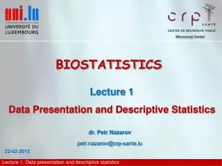
Microarray Center BIOSTATISTICS Lecture 1 Data Presentation and Descriptive Statistics dr. Petr Nazarovpetr.nazarov@crp-sante.lu 22-02-2012

Goal: your FINAL knowledge and skills in biological data analysis ! not marking of your work  Software Data Materials: @ moodle, & • Microsoft® Excel • with Data Analysis Add-In installed http://edu.sablab.net/data/xls http://edu.sablab.net/biostat/2013 COURSE OVERVIEW Organization “Theoretical” course (30h) Theory Explanations to all Common work Practical course (30h) Individual work Individual explanations ? 3 intermediate tests scored 0-3 (9 points in total) Final examination (questions) Final examination (tasks in Excel)

COURSE OVERVIEW Recommended Literature presentationmethodology

Drug discovery Any biological study where numbers are measured or reported Genomics and systems biology Public health COURSE OVERVIEW Introduction BIOSTATISTICS: why and where?

OUTLINE Lecture 1 • Data and statistic • elements, variables and observation • types of data (qualitative and quantitative) and scales (nominal, ordinal, interval, ratio) • Descriptive statistics: tabular and graphical presentation • frequency distribution • pie, bar chart and histogram representation • cumulative distributions • crosstabulation and scatter diagram • Descriptive statistics: numerical measures • measures of location: mean, mode, median, quantiles/quartiles/percentiles • measure of variability: variance, standard deviation, MAD, coefficient of variation • other measures: skewness of distribution • z-score. Chebyshev's theorem. Detection of outliers. • Exploratory analysis. • 5 number summary • box plot • Measure of association between two variables • covariance and correlation coefficient • interpretation of correlation coefficient

DATA AND STATISTICS Elements, variables, and observations, data scales and types

elements variables observation DATA AND STATISTICS Data: Elements, Variables, and Observations Data The facts and figures collected, analyzed, and summarized for presentation and interpretation. Can we consider the “Place” as element?

Nominal scale data use labels or names to identify an attribute of an element. Ex.1: Male, Female Ex.2: Rooms #: 101, 102, 103, … Ordinal scale data exhibit the properties of nominal data and the order or rank of the data is meaningful. Ex.1: Winners: The 1st, 2nd, 3rd places Ex.2: Marks: A, B, C, … Interval scale data demonstrate the properties of ordinal data and the interval between values is expressed in terms of a fixed unit of measure Ex.1: Examination score 0 -100 Ex.2: Internet fame score  Ratio scale data demonstrate all the properties of interval data and the ratio of two values is meaningful. Ex.1: Weight Ex.2: Price DATA AND STATISTICS Data Scales and Types Data scales: Qualitative Quantitative

DATA AND STATISTICS Task: Define the Scales ?

TABULAR AND GRAPHICAL PRESENTATION Frequency distribution, bar and pie charts, histogram, cumulative frequency distribution, scatter plot

Frequency distribution: Relative frequency distribution: Percent frequency distribution: TABULAR AND GRAPHICAL PRESENTATION Frequency Distribution Frequency distribution A tabular summary of data showing the number (frequency) of items in each of several nonoverlapping classes. • In MS Excel use the following functions: • =COUNTIF(data,element)to get number of “elements” found in the “data” area • =SUM(data)to get the sum of the values in the “data” area

TABULAR AND GRAPHICAL PRESENTATION Example: Pancreatitis Study The role of smoking in the etiology of pancreatitis has been recognized for many years. To provide estimates of the quantitative significance of these factors, a hospital-based study was carried out in eastern Massachusetts and Rhode Island between 1975 and 1979. 53 patients who had a hospital discharge diagnosis of pancreatitis were included in this unmatched case-control study. The control group consisted of 217 patients admitted for diseases other than those of the pancreas and biliary tract. Risk factor information was obtained from a standardized interview with each subject, conducted by a trained interviewer. adapted from Chap T. Le, Introductory Biostatistics pancreatitis.xls Pancreatitis patients:

Frequency distribution: Relative frequency distribution: FREQUENCY DISTRIBUTION Relative Frequency Distribution Frequency distribution A tabular summary of data showing the number (frequency) of items in each of several nonoverlapping classes. pancreatitis.xls Relative frequency distribution A tabular summary of data showing the fraction or proportion of data items in each of several nonoverlapping classes. Sum of all values should give 1 Estimation of probability distribution When number of experiments n  , R.F.D.  P.D. • In Excel use the following functions: • =COUNTIF(data,element)to get number of “elements” found in the “data” area • =SUM(data)to get the sum of the values in the “data” area

TABULAR AND GRAPHICAL PRESENTATION Crosstabulation pancreatitis.xls • In Excel use the following steps: • Insert  Pivot Table • Set the range, including the headers of the data • Select output and set layout by drag-and-dropping the names into the table

Try to avoid using in scientific reports. For public/business presentations only! TABULAR AND GRAPHICAL PRESENTATION Bar and Pie Charts pancreatitis.xls • In MS Excel use the following steps: • Insert  Column  Set data range (both columns of Percent freq. distribution) • Insert Pie  Set data range (one columns of Percent freq. distribution)

TABULAR AND GRAPHICAL PRESENTATION Example: Mice Data Series Tordoff MG, Bachmanov AA Survey of calcium & sodium intake and metabolism with bone and body composition data Project symbol:Tordoff3 Accession number: MPD:103 mice.xls 790 mice from different strains http://phenome.jax.org

bins TABULAR AND GRAPHICAL PRESENTATION Histogram The following are weights in grams for 970 mice: mice.xls Sorted weights show that the values are in the 10 – 49.6 grams. Let us divide the weight into the “bins”

TABULAR AND GRAPHICAL PRESENTATION Histogram Now, let us use bin-size = 1 gram • In Excel use the following steps: • Specify the column of bins (interval) upper-limits • Data  Data Analysis  Histrogram  select the input data, bins, and output (Analysis ToolPak should be installed) • use Chart Wizard  Columns to visualize the results

TABULAR AND GRAPHICAL PRESENTATION Scatter Plot Let us look on mutual dependency of the Starting and Ending weights. mice.xls • In Excel use the following steps: • Select the data region • Use Insert XY (Scatter)

NUMERICAL MEASURES Population and sample, measures of location, quantiles, quartiles and percentiles, measures of variability, z-score, detection of outliers, exploration data analysis, box plot, covariation, correlation

SAMPLE m, mean s2variance n number of elements POPULATION µmean 2variance N  number of elements (usually N=∞) mice.xls 790 mice from different strains http://phenome.jax.org All existing laboratory Mus musculus NUMERICAL MEASURES Population and Sample Population parameter A numerical value used as a summary measure for a population (e.g., the population mean , variance 2, standard deviation ) Sample statistic A numerical value used as a summary measure for a sample (e.g., the sample mean m, the sample variance s2, and the sample standard deviation s)

Mode = 23 Median = 23.5 Mean = 31.7 NUMERICAL MEASURES Measures of Location Mean A measure of central location computed by summing the data values and dividing by the number of observations. Median A measure of central location provided by the value in the middle when the data are arranged in ascending order. Mode A measure of location, defined as the value that occurs with greatest frequency.

median = 55 mean = 61 mode = 48 mean median mode NUMERICAL MEASURES Measures of Location mice.xls Female proportion pf = 0.501 • In Excel use the following functions: • = AVERAGE(data) • = MEDIAN(data) • = MODE(data)

Q3 = 39 Q1 = 21 Q2 = 23.5 NUMERICAL MEASURES Quantiles, Quartiles and Percentiles Percentile A value such that at least p% of the observations are less than or equal to this value, and at least (100-p)% of the observations are greater than or equal to this value. The 50-th percentile is the median. Quartiles The 25th, 50th, and 75th percentiles, referred to as the first quartile, the second quartile (median), and third quartile, respectively. • In Excel use the following functions: • =PERCENTILE(data,p)

Variance A measure of variability based on the squared deviations of the data values about the mean. Standard deviation A measure of variability computed by taking the positive square root of the variance. population sample IQR = 18 Variance = 320.2 St. dev. = 17.9 NUMERICAL MEASURES Measures of Variability Interquartile range (IQR) A measure of variability, defined to be the difference between the third and first quartiles. • In Excel use the following functions: • =VAR(data), =STDEV(data)

NUMERICAL MEASURES Measures of Variability Coefficient of variation A measure of relative variability computed by dividing the standard deviation by the mean. CV = 57% Median absolute deviation (MAD) MAD is a robust measure of the variability of a univariate sample of quantitative data.

NUMERICAL MEASURES Measures of Variability Skewness A measure of the shape of a data distribution. Data skewed to the left result in negative skewness; a symmetric data distribution results in zero skewness; and data skewed to the right result in positive skewness. adapted from Anderson et al Statistics for Business and Economics

Ending weight vs. Starting weight sxy= 39.8 hard to interpret NUMERICAL MEASURES Measure of Association between 2 Variables Covariance A measure of linear association between two variables. Positive values indicate a positive relationship; negative values indicate a negative relationship. sample population • In Excel use function: • =COVAR(data) mice.xls

NUMERICAL MEASURES Measure of Association between 2 Variables Correlation (Pearson product moment correlation coefficient) A measure of linear association between two variables that takes on values between -1 and +1. Values near +1 indicate a strong positive linear relationship, values near -1 indicate a strong negative linear relationship; and values near zero indicate the lack of a linear relationship. population sample • In Excel use function: • =CORREL(data) rxy= 0.94 mice.xls

If we have only 2 data points in x andy datasets, what values would you expect for correlation b/w x and y ? NUMERICAL MEASURES Correlation Coefficient Wikipedia

NUMERICAL MEASURES z-score and Detection of Outliers z-score A value computed by dividing the deviation about the mean (xi x) by the standard deviation s. A z-score is referred to as a standardized value and denotes the number of standard deviations xi is from the mean. Chebyshev’s theorem For any data set, at least (1 – 1/z2) of the data values must be within z standard deviations from the mean, where z – any value > 1. • For ANY distribution: • At least 75 % of the values are within z = 2 standard deviations from the mean • At least 89 % of the values are within z = 3 standard deviations from the mean • At least 94 % of the values are within z = 4 standard deviations from the mean • At least 96% of the values are within z = 5 standard deviations from the mean

Example: Gaussian distribution NUMERICAL MEASURES Detection of Outliers • For bell-shaped distributions: • Approximately 68 % of the values are within 1 st.dev. from mean • Approximately 95 % of the values are within 2 st.dev. from mean • Almost all data points are inside 3 st.dev. from mean Outlier An unusually small or unusually large data value. For bell-shaped distributions data points with |z|>3 can be considered as outliers.

NUMERICAL MEASURES Task: Detection of Outliers mice.xls Using Excel, try to identify outlier mice on the basis of Weight change variable For bell-shaped distributions data points with |z|>3 can be considered as outliers. • In Excel use the following functions: • = AVERAGE(data) - mean, m • = STDEV(data) - standard deviation, s • = abs(data) - absolute value • sort by z-scale to identify outliers 

Detection of Outliers Iglewicz-Hoaglin Method Iglewicz-Hoaglin method: modified Z-score These authors recommend that modified Z-scores with an absolute value of greater than 3.5 be labeled as potential outliers. |z|>3.5  outlier Boris Iglewicz and David Hoaglin (1993), "Volume 16: How to Detect and Handle Outliers", The ASQC Basic References in Quality Control: Statistical Techniques, Edward F. Mykytka, Ph.D., Editor More methods are at: http://www.itl.nist.gov/div898/handbook/eda/section3/eda35h.htm

Box plot A graphical summary of data based on a five-number summary Q2 Max Min Q1 Q3 • In Excel use (indirect): • Insert → Other charts → Open-high-low-close 1.5 IQR NUMERICAL MEASURES Exploration Data Analysis Five-number summary An exploratory data analysis technique that uses five numbers to summarize the data: smallest value, first quartile, median, third quartile, and largest value • In Excel use: • Tool → Data Analysis → Descriptive Statistics children.xls Min. : 12 Q1 : 25 Median: 32 Q3 : 46 Max. : 79 Box plot

1. Build 5 number summaries for males and females 2. Combine the numbers into the following order • In Excel use: • Insert → Other charts → Open-high-low-close • Put “series-in-rows” • Adjust colors, etc NUMERICAL MEASURES Example: Mice Weight Example Build a box plot for weights of male and female mice mice.xls

As an example of the need of weighted mean, consider the following sample of five purchases of a raw material over several months Note that the cost per pound varies from $2.80 to $3.40, and quantity purchased has varied from 500 to 2750. Suppose that manager asked for information about the mean cost per pound of the raw material. If we would use a simple mean of the cost p.p.: we overestimate the average cost! NUMERICAL MEASURES Weighted Mean Weighted mean The mean obtained by assigning each observation a weight that reflects its importance Anderson et al Statistics for Business and Economics

Mean for grouped data Variance for grouped data NUMERICAL MEASURES Grouped Mean Grouped data Data available in class intervals as summarized by a frequency distribution. Individual values of the original data are not available. children.xls not available

QUESTIONS ? Thank you for your attention to be continued…

Detection of Outliers Grubbs' Test Grubbs' test is an iterative method to detect outliers in a data set assumed to come from a normally distributed population. (k) – iteration k m – mean of the rest data s – st.dev. of the rest data Grubbs' statisticsat step k+1: The hypothesis of no outliers is rejected at significance level α if More methods are at: http://www.itl.nist.gov/div898/handbook/eda/section3/eda35h.htm

Detection of Outliers Grubbs' Test Let's perform Grubb's test for "Weight change" of mice.xls Step 1. Generate critical value N: =COUNTIF(A:A,">=0") t2: =TINV(0.05/(2*E1),E1-2)^2 GCrit = (E1-1)/SQRT(E1)* SQRT(E2/(E1-2+E2)) Step 2. Build |z| and sort in descending order Step 3. If the first |z| value is > GCrit – remove it and go to step 2, else finish.

Microarray Center