Descriptive Statistics Numerical Methods
Descriptive Statistics Numerical Methods. Measures of Central Location Measures of Variability Measures of Relative Position. Numerical Measures of Central Location. Mean Median Mode Weighted Mean. Numerical Measures of Central Location Mean.

Descriptive Statistics Numerical Methods
E N D
Presentation Transcript
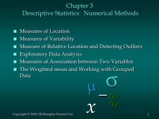
Descriptive StatisticsNumerical Methods Measures of Central Location Measures of Variability Measures of Relative Position
Numerical Measures of Central Location Mean Median Mode Weighted Mean
Numerical Measures of Central LocationMean The mean of a data set is the average of all the data values. The mean of a sample of n measurements is denoted by and equals If the data are from a population, the mean is denoted by (mu) and equals
Numerical Measures of Central LocationMedian The median of a data set is the value in the middle when the data items are arranged in ascending order. For an odd number of observations, the median is the middle value. For an even number of observations, the median is the average of the two middle values.
Numerical Measures of Central LocationMode The mode of a data set is the value that occurs with greatest frequency. The greatest frequency can occur at two or more different values. If the data have exactly two modes, the data are bimodal. If the data have more than two modes, the data are multimodal.
Mean, Median, and ModeExample: Problem #2.64, p. 70 Mean: =7+11+8+(-6)+4+0+4+12=40 The mean of the sample is 5.
Mean, Median, and ModeExample: Problem #2.64, p. 70 Median First step: arrange data in ascending order. -6, 0, 4, 4, 7, 8, 11, 12 Second step: find the middle value. Md=(4+7)/2=5.5 The median of the sample is 5.5.
Mean, Median, and ModeExample: Problem #2.64, p. 70 Mode A value that occurs more often than any of the others is 4. The mode is 4 since this occurs twice.
Numerical Measures of Central Location Weighted Mean The weighted mean of a set of measurements with relative weights is given by
Weighted Mean Example: Problem #2.75, p. 72 Weighted mean The student’s grade point average for the semester is 2.73.
Numerical Measures of Variability Range Variance Standard Deviation
Numerical Measures of Variability Range The range of a data set is the difference between the largest and smallest data values. It is the simplest measure of variability. It is very sensitive to the smallest and largest data values.
Numerical Measures of Variability Variance The variance is a measure of variability that utilizes all the data. It is based on the difference between the value of each observation (xi) and the mean ( for a sample, for a population).
Numerical Measures of Variability Variance The variance is the average of the squared differences between each data value and the mean. If the data set is a sample, the variance is denoted by s2. If the data set is a population, the variance is denoted by 2.
Numerical Measures of Variability Shortcut Formula for Variance We will be using a shortcut formula to determine the variance. First, find SS(x) using the formula Then, calculate the sample variance using the formula
Numerical Measures of Variability Standard Deviation • The standard deviation of a data set is the positive square root of the variance. • It is measured in the same units as the data, making it more easily comparable, than the variance, to the mean. • If the data set is a sample, the standard deviation is denoted by s. • If the data set is a population, the standard deviation is denoted by (sigma).
Range, Variance, and Standard DeviationExample: Problem #2.85, p. 82 Range Range = Largest value – Smallest value = 9 – 0 = 9 The range is 9.
Range, Variance, and Standard DeviationExample: Problem #2.85, p. 82 Variance First step: find and
Range, Variance, and Standard DeviationExample: Problem #2.85, p. 82 Variance Second step: find SS(x) using the shortcut formula
Range, Variance, and Standard DeviationExample: Problem #2.85, p. 82 Variance Third step: calculate the sample variance by using the following formula The sample variance is 13.5.
Range, Variance, and Standard DeviationExample: Problem #2.85, p. 82 Standard deviation The sample standard deviation is 3.7.
Understanding the Significance of Standard Deviation The standard deviation is the most common way of measuring the variation in a data set. For two data sets, the one that has the greater variability will have the larger standard deviation. The standard deviation is also useful in describing a single distribution of measurements. This description will be accomplished by examining two statements – the Empirical Rule and Chebyshev’s Theorem.
The Empirical Rule If a set of measurements has a mound –shaped distribution, then The interval from to will contain approximately 68% of the measurements. The interval from to will contain approximately 95% of the measurements. The interval from to will contain approximately all the measurements.
The Empirical RuleExample: Problem #2.107, p. 91 For this problem, use the Empirical Rule to describe the distribution of weights. Solution: Since the distribution of weights is mound shaped, it is reasonable to assume that the Empirical Rule is applicable in this situation. Therefore, we can expect that:
The Empirical RuleExample: Problem #2.107, p. 91 Approximately 68% of the loaves have weights falling in the interval , i.e., from 27.2 to 28.8 ounces. Approximately 95% of the loaves have weights falling in the interval , i.e., from 26.4 to 29.6 ounces. Approximately all of the loaves have weights falling in the interval , i.e., from 25.6 to 30.4 ounces.
Chebyshev’s Theorem For any set of measurements and any number k1, the interval from to will contain at least (1 - 1/k2)*100% of the measurements. Chebyshev’s Theorem applies to all possible distributions. It is very conservative. Chebyshev’s Theorem gives the minimum proportion of the measurements that will lie within k standard deviation of their mean.
Chebyshev’s Theorem For instance: At least 75% of the items must be within k = 2 standard deviations of the mean. At least 89% of the items must be within k = 3 standard deviations of the mean. At least 90% of the items must be within k = 3.5 standard deviations of the mean.
Chebyshev’s TheoremExample: Problem #2.108, p.91 Solution: According to Chebyshev’s Theorem, at least (1 - 1/k2)*100% measurements lie within the interval Then, 96% = (1 - 1/k2)*100% k=5 Therefore, at least 96% of the measurements lie within the interval i.e., 96% of the capsules will contain from 492 to 522 grams of vitamin C.
Measures of Relative Position Z-Scores Percentiles 5-Number Summaries Boxplots
Measures of Relative Position Z-Scores The z-score is often called the standardized value. It denotes the number of standard deviations a data value x is from the mean. A data value less than the sample mean will have a z-score less than zero. A data value greater than the sample mean will have a z-score greater than zero. A data value equal to the sample mean will have a z-score of zero.
Measures of Relative Position Percentiles For a large set of measurements, the percentiles are denoted by P1, P2, P3, . . . , P99. Pkis called thekthpercentile and is the value such that approximately k% of the measurements are less and (100-k)% are more. Three frequently used percentiles are P25, P50, and P75.They are called the first, second, and thirdquartiles, respectively, and are denoted by Q1, Q2, and Q3.
PercentilesExample: Problem #2.121, p. 100 Approximately 50% of scores on the test are between 104 and 195. Approximately 75% of scores on the test are above 104. Approximately 25% of scores on the test are above 195.
Measures of Relative Position 5-Number Summaries The 5-number summaries of a set of measurements are the values • Smallest Value • First Quartile • Second Quartile (Median) • Third Quartile • Largest Value
Measures of Relative Position Boxplots The simplest boxplot consists of a pictorial display of a distribution’s 5-number summary. The boxplot provides us with a visual impression of how a distribution’s values are spread out from their median value Q2.
Measures of Relative Position Boxplots The box is drawn above the real number line such that: the ends of the box are at the first and third quartiles; a vertical line is drawn in the box at the location of the median; and lines are drawn from the ends of the box to the smallest and largest data values (the lines are called whiskers).