Noise-Insensitive Boolean-Functions are Juntas
620 likes | 802 Vues
Noise-Insensitive Boolean-Functions are Juntas. Guy Kindler & Muli Safra. Dictatorship. Def : a boolean function P([n]) {-1,1} is a monotone e - dictatorships --denoted f e --if:. We would tend to omit p. Juntas.

Noise-Insensitive Boolean-Functions are Juntas
E N D
Presentation Transcript
Noise-Insensitive Boolean-Functions are Juntas Guy Kindler & Muli Safra
Dictatorship Def: a boolean function P([n]){-1,1} is a monotone e-dictatorships --denoted fe--if:
We would tend to omit p Juntas Def: a boolean function f:P([n]){-1,1} is a j-Junta if J[n] where|J|≤ j, s.t. for every x[n]: f(x) = f(x J) Def: f is an [, j]-Junta if j-Junta f’ s.t. Def: f is an [, j, p]-Junta if j-Junta f’ s.t.
Codes and Boolean Functions Def: a code is a mapping of a set of n elements (log n bits’ string) to a set of m-bits strings C:[n]{0,1}m, i.e. C(e) = a1…am Def: Let Sj={e[n] | C(e)j=T} Let ={Sj}j[m] C(1) C(2) C(3) C(n) FF TTF F TT F TT T Sm={1,n} S1={2,3,n}
Codes and Boolean Functions C(1) C(2) C(3) C(n) FF0 TTF F TT F TT T Def: Let Ee be the encodingof element e. • Consider {Ee}e[n]Each Ee’s truth-table represents a legal--code-word of C( since C(e) = Ee(S1)…Ee(Sm) ) Sm={1,n} S1={2,3,n}
Long-Code • In the long-code L:[n] {0,1}2neach element is encoded by an 2n-bits • This is the most extensive code, as = P([n]), i.e. the bits represent all subsets in P([n])
Long-Code • Encoding an element e[n]: • Eelegally-encodes an element e if Ee = fe T F F T T
Motivation – Testing Long-code • Def (a long-code test): given a code-word w, probe it in a constant number of entries, and • accept w.h.p if w is a monotone dictatorship • reject w.h.p if w is not close to any monotone dictatorship
Motivation – Testing Long-code • Def(a long-code list-test): given a code-word w, probe it in a constant number of entries, and • accept w.h.p if w is a monotone dictatorship, • reject w.h.p if wis not even approximately determined by a small list of domain elements, that is, if a JuntaJ[n] s.t. f is close to f’ and f’(x)=f’(xJ) for all x • Note: a long-code list-test, distinguishes between the case w is a dictatorship, to the case w is far from a junta.
Motivation – Testing Long-code • The long-code test, and the long-code list-test are essential tools in proving hardness results. Examples … • Hence finding simple sufficient-conditions for a function to be a junta is important.
Background • Thm (Friedgut): a boolean function f with small average-sensitivity is an [,j]-junta • Thm (Bourgain): a boolean function f with small high-frequency weight is an [,j]-junta • Thm (Kindler&Safra): a boolean function f with small high-frequency weight in a p-biased measure is an [,j]-junta • Corollary: a boolean function f with smallnoise-sensitivity is an [,j]-junta • Parameters: average-sensitivity, high-frequency weight, noise-sensitivity
Noise-Sensitivity • Idea: check how the value of f changes when the input is changed not on one, but on several coordinates. [n] I z x
[n] I z x Noise-Sensitivity • Def(,p,x[n] ): Let 0<<1, and xP([n]). Then y~,p,x, if y = (x\I) z where • I~[n] is a noise subset, and • z~ pI is a replacement. Def(-noise-sensitivity): let 0<<1, then • Note: deletes a coordinate in x w.p. (1-p), adds a coordinate to x w.p. p. Hence, when p=1/2: equivalent to flipping each coordinate in x w.p. /2.
Noise-Sensitivity – Cont. • Advantage: very efficiently testable (using only two queries) by a perturbation-test. • Def(perturbation-test): choose x~p, and y~,p,x, check whether f(x)=f(y).The success is proportional to the noise-sensitivity of f. • Prop: the -noise-sensitivity is given by
Relation between Parameters • Prop: small ns small high-freq weight • Proof: therefore: if ns is small, then Hence the high frequencies must have small weights (as ). • Prop: small as small high-freq weight • Proof:
Average and Restriction [n] Def: Let I[n],xP([n]\I), the restriction function is Def: the average function is Note: I y x [n] I y y y y y x
Fourier Expansion • Prop: • Prop: • Corollary:
Variation Def: the variation of f(formerly called influence): Prop: the following are equivalent definitions to the variation of f:
Proof • Recall • Therefore
Proof – Cont. • Recall • Therefore (by Parseval):
High/Low Frequencies and their Weights Def: the high-frequency portion of f: Def: the low-frequency portion of f: Def: the high-frequency-weight is: Def: the low-frequency-weight is:
Low-freq variation and Low-freq average-sensitivity Def: the low-frequency variation is: Def: the average sensitivity is And in Fourier representation: Def: the low-frequency average sensitivity is:
Main Results Theorem: constant >0 s.t. any boolean function f:P([n]){-1,1} satisfying is an [,j]-junta for j=O(-2k32k). Corollary: fix a p-biased distribution p overP([n]). Let >0 be any parameter. Set k=log1-(1/2). Then constant >0 s.t. any boolean function f:P([n]){-1,1} satisfying is an [,j]-junta for j=O(-2k32k).
First Attempt: Following Freidgut’s Proof Thm: any boolean function f is an [,j]-junta for Proof: • Specify the juntawhere, let k=O(as(f)/) and fix =2-O(k) • Show the complement of J has small variation P([n]) J
P([n]) J Following Freidgut - Cont Lemma: Proof: Now, lets bound each argument: Prop: Proof: characters of sizek contribute to the average-sensitivity at least (since )
we do not know whether as(f) is small! True only since this is a {-1,0,1} function. So we cannot proceed this way with only ask! Following Freidgut - Cont Prop: Proof:
Important Lemma • Lemma: >0, s.t. for any and any function g:P([m]) , the following holds: high-freq Low-freq
Beckner/Nelson/Bonami Inequality Def: let Tbe the following operator on any f, Thm: for any p≥rand≤((r-1)/(p-1))½ Corollary: for f s.t. f>k=0
Probability Concentration • Simple Bound: • Proof: • Low-freq Bound: Let g:P([m]) s.t. g>k=0, let >0, then >0 s.t. • Proof: recall the corollary:
Lemma’s Proof • Now, let’s prove the lemma: • Bounding low and high freq separately:, simple bound Low-freq bound
Shallow Function • Def: a function f is linear, if only singletons have non-zero weight • Def: a function f is shallow, if f is either a constant or a dictatorship. • Claim: boolean linear functions are shallow. weight Charactersize 0 1 2 3 k n
Boolean Linear Shallow • Claim: boolean linear functions are shallow. • Proof: let f be boolean linear function, we next show: • {io} s.t. (i.e. ) • And conclude, that either or i.e.f is shallow
1 -1 Claim 1 • Claim 1: let f be boolean linear function, then {io} s.t. • Proof: w.l.o.g assume • for any z{3,…,n}, considerx00=z, x10=z{1}, x01=z{2}, x11=z{1,2} • then . • Next value must be far from {-1,1}, • A contradiction! (boolean function) • Therefore ?
1 0 -1 Claim 2 • Claim 2: let f be boolean function, s.t.Then either or • Proof: consider f() and f(i0): • Then • but f is boolean, hence • therefore
Proving FKN: almost-linear close to shallow • Theorem: Let f:P([n]) be linear, • Let • let i0 be the index s.t. is maximal then • Note: f is linear, hence w.l.o.g., assume i0=1, then all we need to show is:We show that in the following claim and lemma.
Corollary • Corollary: Let f be linear, andthen a shallow booleanfunction g s.t. • Proof: let , let g be the boolean function closest to l. Then,this is true, as • is small (by theorem), • and additionally is small, since
weight Each of weight no more than c Characters {} {1} {2} {i} {n} {1,2} {1,3} {n-1,n} S {1,..,n} Claim 1 • Claim 1: Let f be linear. w.l.o.g., assumethen global constant c=min{p,1-p}s.t.
1 -1 Proof of Claim1 • Proof: assume • for any z{3,…,n}, considerx00=z, x10=z{1}, x01=z{2}, x11=z{1,2} • then • Next value must be far from {-1,1} ! • A contradiction! (to ) ?
note Lemma • Lemma: Let g be linear, let assume , then • Corrolary: The theorem follows from the combination of claim1 and the lemma: • Let m be the minimal index s.t. • Consider • If m=2: the theorem is obtained (by lemma) • Otherwise -- a contradiction to minimality of m :
Lemma’s Proof • Lemma’s Proof: Note • Hence, all we need to show is that • Intuition: • Note that |g| and |b| are far from 0(since |g| is -close to 1, and c-close to b). • Assumeb>0, then for almost all inputs x, g(x)=|g(x)| (as ) • Hence E[g] E[|g(x)|], and • therefore var(g) var(|g|)
Proof-map: |g|,|b| are far from 0 g(x)=|g(x)| for almost all x E[g] E[|g|] var(g) var(|g|) • E2[g] - E2[|g|] = 2E2[|g|1{f<0}] o() (by Azuma’s inequality) • We next show var(g) var(|g|): • By the premise • however • therefore
Central Ideas: Linear Functions and Random Partition Idea 1: recall • (theorem’s premise) • Assume f is close to linear then f is close to shallow (by [FKN]). Idea 2: Let . • Partition J into I1,…,Ir. • r is large, hence w.h.p fI[x] is close to linear(low freq characters intersect each I by 1 element). P([n]) I2 Ir I I1 J
P([n]) Variation Lemma I2 Ir I I1 • Lemma(variation): >0, and r>>k s.t. • Corollary: for most I and x, fI[x] is almost constant J
P([n]) Using Idea2 I2 Ir I I1 • By union bound on I1,…,Ir: • (set ) • Let f’(x) = sign( AJ[f](xJ) ). f’ is the boolean function closest to AJ[f], therefore • Hence f is an [,j]-junta. J
variation-Lemma - Proof Plan Lemma(variation): >0, and r>>k s.t. Sketch for proving the variation lemma: • w.h.p fI[x] is almost linear • w.h.p fI[x] is close to shallow • fI[x] cannot be close to dictatorship too often.
Proof-map: • w.h.p fI[x]is almost linear • w.h.pfI[x]is close to shallow • fI[x]cannot be close todictatorshiptoo often. Lemma Proof The low frequencies characters are small, r is rather large, hence w.h.p the characters are linear at each I. P([n]) I2 Ir I I1 J
Proof-map: • w.h.p fI[x]is almost linear • w.h.pfI[x]is close to shallow • fI[x]cannot be close todictatorshiptoo often. almost linear almost shallow Theorem([FKN]): global constant M, s.t. boolean function f, shallow boolean function g, s.t. • Hence, ||fI[x]>1||2 is small fI[x] is close to shallow!
Preliminary Lemma and Props • Prop: if fI[x] is a dictatorship, then coordinate i s.t. (where p is the bias). • Corollary (from [FKN]): global constant M, s.t. boolean function h, eitheror weight Total weight of no more than 1-p Characters {1} {2} {i} {n} {1,2} {1,3} {n-1,n} S {1,..,n}
Proof-map: • w.h.p fI[x]is almost linear • w.h.pfI[x]is close to shallow • fI[x]cannot be close todictatorshiptoo often. Few Dictatorships • Lemma: >0, s.t. for any and any function g:P([m]) , the following holds: • Def: Let DI be the set of xP(I), s.t. fI[x] is a dictatorship, i.e. • Next we show, that |DI| must be small, hence for most x, fI[x] is constant.
Parseval Prev lemma |DI| must be small • Lemma: • Proof: let , then Each S is counted only for one index iI. (Otherwise, if S was counted for both i and j in I, then |SI|>1!)