How to learn hard Boolean functions
How to learn hard Boolean functions. Włodzisław Duch Department of Informatics, Nicolaus Copernicus University , Toru ń , Poland School of Computer Engineering, Nanyang Technological University, Singapore Google: Duch Poliopt imization , 6/ 200 6. Plan.

How to learn hard Boolean functions
E N D
Presentation Transcript
How to learnhard Boolean functions Włodzisław Duch Department of Informatics, Nicolaus Copernicus University, Toruń, Poland School of Computer Engineering, Nanyang Technological University, Singapore Google: Duch Polioptimization, 6/2006
Plan • Problem: learning systems are not able to learn almost any functions! Learning = adaptation of model parameters. • Linear discrimination, Support Vector Machines and kernels. • Neural networks. • What happens in hidden space? • k-separability • How to learn any function?
GhostMiner Philosophy GhostMiner, data mining tools from our lab + Fujitsu: http://www.fqspl.com.pl/ghostminer/ • Separate the process of model building (hackers) and knowledge discovery, from model use (lamers) => GhostMiner Developer & GhostMiner Analyzer • There is no free lunch – provide different type of tools for knowledge discovery: decision tree, neural, neurofuzzy, similarity-based, SVM, committees. • Provide tools for visualization of data. • Support the process of knowledge discovery/model building and evaluating, organizing it into projects. • We are building completely new tools ! Surprise! Almost nothing can be learned using such tools!
Easy and difficult problems Linear separation: good goal if simple topological deformation of decision borders is sufficient. Linear separation of such data is possible in higher dimensional spaces; this is frequently the case in pattern recognition problems. RBF/MLP networks with one hidden layer solve such problems. Difficult problems: disjoint clusters, complex logic. Continuous deformation is not sufficient; networks with localized functions need exponentially large number of nodes. This is typical in AI problems, real perception, object recognition, text analysis, bioinformatics, logical problems ... Boolean functions: for n bits there are K=2n binary vectors that can be represented as vertices of n-dimensional hypercube. Each Boolean function is identified by K bits. BoolF(Bi) = 0 or 1 for i=1..K, for 2KBoolean functions. Ex: n=2 functions, vectors {00,01,10,11}, Boolean functions {0000, 0001 ... 1111}, decimal numbers 0 to 15.
For normalized data Xi [0,1] FDA projection is close to the lattice projection, defined as W1=[1,1,..1] direction and W2 maximizing separation of the points with fixed number of 1 bits. Lattice projection for n=3, 4 Projection on 111 ... 111 gives clusters with 0, 1, 2 ... n bits.
Boolean functions n=2, 16 functions, 12 separable, 4 not separable. n=3, 256 f, 104 separable (41%), 152 not separable. n=4, 64K=65536, only 1880 separable (3%) n=5, 4G, but << 1% separable ... bad news! Existing methods may learn some non-separable functions, but most functions cannot be learned ! Example: n-bit parity problem; many papers in top journals. No off-the-shelf systems are able to solve such problems. For all parity problems SVM is below base rate! Such problems are solved only by special neural architectures or special classifiers – if the type of function is known. Ex: parity problems are solved by
Linear discrimination In the feature space X find direction W that separates data into g(X)= WX > q, with fixed W, defines a half-space. g(X)=+1 g(X)> +1 y=W.X g(X)=-1 1/||W|| g(X)< -1 Frequently a single hyperplane (projection on a line) is sufficient to separate data, if not find a better space (usually more features).
LDA in larger space Use LDA, just add some new dimensions!Add to inputXi2, and products XiXj, as new features. Example: 2D => 5D case {X1, X2, X12, X22, X1X2} But the number of such tensor products grows exponentially. Suppose that strongly non-linear borders are needed. Fig. 4.1 Hasti et al.
How to add new dimensions? In the space defined by data expand W in input vectors: Makes sense, since a component WZ of W=WZ+WX that does not belong to the space spanned by X(i) vectors has no influence on the discrimination process, because WZTX=0. Insert W in the discriminant function: Transform X to a new space Great! Discriminant g(X) has not changed, except that K is now defined in the F space. F is not needed, just a scalar product K(X,X’), called “kernel”.
Maximization of margin Among all discriminating hyperplanes there is one defined by support vectors that is clearly better.
SVM SVM = LDA in the space defined by kernels + optimization that includes maximization of margins (min. of ||W||), focusing on vectors close to decision borders. Problem for Bayesian statistics: what data should be used for training? Local priors and conditional distributions work better, but how local should they be? SVM: discrimination based on cases close to decision border. Kernels may be sophisticated procedures to evaluate similarity of texts, molecules, DNA strings etc. Any method may be improved by moving to a kernel space! Even random projection to high-dim. space works well.
Gaussian kernels Gaussian kernels work quite well, giving for Gaussian mixtures close to optimal Bayesian errors. Solution requires continuous deformation of decision borders and is therefore rather easy. 4-deg. polynomial kernel is slightly worse then a Gaussian kernel, C=1. In the kernel space decision borders are flat!
Neural networks: thyroid screening Clinical findings Finaldiagnoses Hidden units Age sex … … Normal Hypothyroid TSH Hyperthyroid T4U T3 TT4 TBG Garavan Institute, Sydney, Australia 15 binary, 6 continuous Training: 93+191+3488 Validate: 73+177+3178 • Determine important clinical factors • Calculate prob. of each diagnosis.
Learning in neural networks • MLP/RBF: first fast MSE reduction, very slow later. Typical MSE(t) learning curve: after 10 iterations almost all work is done, but the final convergence is achieved only after a very long process, about 1000 iterations. What is going on?
Learning trajectories • Take weights Wi from iterations i=1..K; PCA on Wicovariance matrix captures 95-95% variance for most data, so error function in 2D shows realistic learning trajectories. Papers by M. Kordos & W. Duch Instead of local minima large flat valleys are seen – why? Data far from decision borders has almost no influence, the main reduction of MSE is achieved by increasing ||W||, sharpening sigmoidal functions.
Selecting Support Vectors Active learning: if contribution to the parameter change is negligible remove the vector from training set. If the difference is sufficiently small the pattern X will have negligible influence on the training process and may be removed from the training. Conclusion: select vectors with eW(X)>emin, for training. 2 problems: possible oscillations and strong influence of outliers. Solution: adjust emin dynamically to avoid oscillations; remove also vectors with eW(X)>1-emin=emax
SVNT algorithm Initialize the network parameters W, set De=0.01,emin=0, set SV=T. Until no improvement is found in the last Nlast iterations do • Optimize network parameters for Nopt steps on SV data. • Run feedforward step on T to determine overall accuracy and errors, take SV={X|e(X) [emin,1-emin]}. • If the accuracy increases: compare current network with the previous best one, choose the better one as the current best • increase emin=emin+De and make forward step selecting SVs • If the number of support vectors |SV| increases: decrease emin=emin-De; decrease De = De/1.2 to avoid large changes
Satellite image data Multi-spectral values of pixels in the 3x3 neighborhoods in section 82x100 of an image taken by the Landsat Multi-Spectral Scanner; intensities = 0-255, training has 4435 samples, test 2000 samples. Central pixel in each neighborhood is red soil (1072), cotton crop (479), grey soil (961), damp grey soil (415), soil with vegetation stubble (470), and very damp grey soil (1038 training samples). Strong overlaps between some classes. System and parameters Train accuracy Test accuracy SVNT MLP, 36 nodes, a=0.5 96.5 91.3 SVM Gaussian kernel (optimized) 91.6 88.4 RBF, Statlog result 88.9 87.9 MLP, Statlog result 88.8 86.1 C4.5 tree 96.0 85.0
Hypothyroid data 2 years real medical screening tests for thyroid diseases, 3772 cases with 93 primary hypothyroid and 191 compensated hypothyroid, the remaining 3488 cases are healthy; 3428 test, similar class distribution. 21 attributes (15 binary, 6 continuous) are given, but only two of the binary attributes (on thyroxine, and thyroid surgery) contain useful information, therefore the number of attributes has been reduced to 8. Method % train % test C-MLP2LN rules 99.89 99.36 MLP+SCG, 4 neurons 99.81 99.24 SVM Minkovsky opt kernel 100.0 99.18 MLP+SCG, 4 neur, 67 SV 99.95 99.01 MLP+SCG, 4 neur, 45 SV 100.0 98.92 MLP+SCG, 12 neur. 100.0 98.83 Cascade correlation 100.0 98.5 MLP+backprop 99.60 98.5 SVM Gaussian kernel 99.76 98.4
What feedforward NN really do? Vector mappings from the input space to hidden space(s) and to the output space. Hidden-Output mapping done by perceptrons. A single hidden layer case is analyzed below. T= {Xi}training data, N-dimensional. H = {hj(Xi)}Ximage in the hidden space, j=1 .. NH-dim. Y = {yk{h(Xi)}Ximage in the output space, k=1 .. NC-dim. ANN goal: scatterograms of T in the hidden space should be linearly separable; internal representations will determine network generalization capabilities and other properties.
What happens inside? Many types of internal representations may look identical from outside, but generalization depends on them. • Classify different types of internal representations. • Take permutational invariance into account: equivalent internal representations may be obtained by re-numbering hidden nodes. • Good internal representations should form compact clusters in the internal space. • Check if the representations form separable clusters. • Discover poor representations and stop training. • Analyze adaptive capacity of networks. • .....
RBF for XOR Is RBF solution with 2 hidden Gaussians nodes possible? Typical architecture: 2 input – 2 Gauss – 2 linear. Perfect separation, but not a linear separation! 50% errors. Single Gaussian output node solves the problem. Output weights provide reference hyperplanes (red and green lines), not the separating hyperplanes like in case of MLP. Output codes (ECOC): 10 or 01 for green, and 00 for red.
3-bit parity For RBF parity problems are difficult; 8 nodes solution: 1) Output activity; 2) reduced output, summing activity of 4 nodes. 3) Hidden 8D space activity, near ends of coordinate versors. 4) Parallel coordinate representation. 8 nodes solution has zero generalization, 50% errors in tests.
3-bit parity in 2D and 3D Output is mixed, errors are at base level (50%), but in the hidden space ... Conclusion: separability is perhaps too much to desire ... inspection of clusters is sufficient for perfect classification; add second Gaussian layer to capture this activity; just train second RBF on this data (stacking)!
Goal of learning Linear separation: good goal if simple topological deformation of decision borders is sufficient. Linear separation of such data is possible in higher dimensional spaces; this is frequently the case in pattern recognition problems. RBF/MLP networks with one hidden layer solve the problem. Difficult problems: disjoint clusters, complex logic. Continuous deformation is not sufficient; networks with localized functions need exponentially large number of nodes. This is typical in AI problems, real perception, object recognition, text analysis, bioinformatics ... Linear separation is too difficult, set an easier goal. Linear separation: projection on 2 half-lines in the kernel space: line y=WX, with y<0 for class – and y>0 for class +. Simplest extension: separation into k-intervals. For parity: find direction W with minimum # of intervals, y=W.X
s(W.X+q1) X1 +1 y=W.X +1 X2 s(W.X+q2) +1 -1 X3 +1 +1 +1 X4 -1 s(W.X+q4) k-separability Can one learn all Boolean functions? Problems may be classified as 2-separable (linear separability); non separable problems may be broken into k-separable, k>2. Neural architecture for k=4 intervals. Blue: sigmoidal neurons with threshold, brown – linear neurons.
k-sep learning Try to find lowest k with good solution, start from k=2. • Assume k=2 (linear separability), try to find good solution; • if k=2 is not sufficient, try k=3; two possibilities are C+,C-,C+ and C-, C+, C-this requires only one interval for the middle class; • if k<4 is not sufficient, try k=4; two possibilities are C+, C-, C+, C-and C-, C+, C-, C+this requires one closed and one open interval. Network solution is equivalent to optimization of specific cost function. Simple backpropagation solved almost all n=4 problems for k=2-5 finding lowest k with such architecture!
A better solution? What is needed to learn Boolean functions? • cluster non-local areas in the X space, use W.X • capture local clusters after transformation, use G(W.X-q) SVM cannot solve this problem! Number of directions W that should be considered grows exponentially with size of the problem n. Constructive neural network solution: • Train the first neuron using G(W.X-q) transfer function on whole data T, capture the largest pure cluster TC . • Train next neuron on reduced data T 1=T-TC • Repeat until all data is handled; they creates transform. X=>H • Use linear transformation H => Y for classification.
Summary • Difficult learning problems arise when non-connected clusters are assigned to the same class. • No off-shelf classifiers are able to learn difficult Boolean functions. • Visualization of activity of the hidden neurons shows that frequently perfect but non-separable solutions are found despite base-rate outputs. • Linear separability is not the best goal of learning, other targets that allow for easy handling of final non-linearities should be defined. • Simplest extension is to isolate non-linearity in form of k intervals. • k-separability allows to break non-separable problems into well defined classes. • For Boolean problems k-separability finds simplest data model with linear projection and k parameters defining intervals. • Tests with simplest backpropagation optimization learned difficult Boolean functions. • k-separability may be used in kernel space. Prospects for systems that will learn all Boolean functions are good!
Thank youfor lending your ears ... Google: Duch => Papers