
Technology Mapping
E N D
Presentation Transcript
Technology Mapping Shubham Rai AkashKumar
Outline • Introduction to Technology mapping • Different steps involved in technology mapping • Two main matching strategies • Structural matching • Boolean matching • FPGA technology mapping
Introduction • Technology mapping is the final phase of the logic synthesis. • The previous phases are technology independent. • Technology mapping’s goal is to convert the logic design into a synthesizable schematic. RTL Logic minimization and optimization Technology mapping Verify Schematic
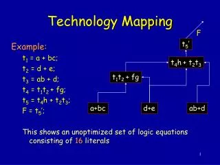
Technology Mapping • Implements the technology independent network by matching pieces of the network with the logic cells that are available in a technology-dependent cell library. • Process of binding nodes in the network to cells in the library. • While performing technology mapping, the algorithm attempts to minimize area, while meeting other user constraints. What kind of other constraints ?
Technology Mapping - General • Library Based Technology Mapping • Standard cell design • A limited set of pre-designed cells • FPGA Technology Mapping • Look-up Table based: each LUT can implement a large no. of functions, e.g., all functions of 5 inputs and 1 output, e.g. in Xilinx FPGAs. • Multiplexer based: each FPGA cell consists of a number of multiplexers e.g. in Actel FPGAs. Why Multiplexers ?
Technology Mapping – Library Based • Standard cells based designs • Library cells are limited: • Library design costs. • Delay / Power / Reliability limits. • Impedance / Capacitance limits.
Cell Library – example Taken from IBM journal of R&D
Cell Library – example • IBM Standard-cell library used for the POWER4. • These 2132 cells are just the basic library but only 12 gate types! • Other gates used • XOR/XNOR (mainly for muxes and comparators) • There are also large buffer, latch / FF libraries • The really tough cases are handled by custom made cells.
Cell Library – example • Ignoring the beta ratios, dual Vt, Gate strength • The designer has the following gates drawn to choose from INV AOI22 NAND2 NAND3 OAI21 NOR2 OAI22 AOI21
Standard cells – AOI22 Icon Diagram Truth Table IN A0 IN OUT Y A1 IN B0 IN B1 AOI22 (technology)
Technology Mapping – Flow • Translates logic equations into a network of technology cells. • Transforms each and every cell in the network. • A three step procedure • Decomposition. • Partitioning. • Matching and Covering. • Often, stages are merged or split in some books and tools
Technology Mapping – Flow • Decomposition • Restructures the Boolean function into the subject graph • Partitioning • Partitions the big network into sub-networks • Matching and Covering • Finds matches between patterns and regions of cells in the subject graph • Uses patterns to cover the subject graph and minimize the cost function
Logic Decomposition • Creating a new representation of the circuit. • Decomposing the network into new primitives. • Most common choice is NAND2 and INV. • The library cells must be decomposed too.
Logic Decomposition – Example • Base Functions: • Pattern Trees: inv1 nand2 nor2 nand3 oai21
Logic Decomposition - Example • These two decompositions match the NAND4 gate. • Not identical for timing issues. • Complex gates can be matched by completely different patterns. • Optimization possibilities. • Common solution – Make all trees left or right oriented. NAND4
Partitioning • Breaking the big network into smaller sub-networks • Each sub-network defined as a subject Boolean graph • Reduce to many multi-input, single-output networks • Reduces the size of the covering problem • Decomposition and partitioning are heuristics • Reduce problem difficulty • Hurt the quality of the final solution
Partitioning • Algorithm • Mark the vertices with multiple out degrees. • Edges whose tails are marked as vertices define the partition boundary. • The above steps convert the original graph to multiple-input single-output subject graphs. • If there are too many inputs, each subject graph can be further partitioned
Pattern Matching and Covering • One of the crucial tasks for technology mapping • Determines which cells in the library may be used to implement a set of nodes in the subject Boolean network.1 • Two main types of pattern matching • Structural matching • Boolean matching [1] A new structural pattern matching algorithm for technology mapping Zhao, M.; Sapatnekar, S.S. , Design Automation Conference, 2001. Page(s): 371 -376
Structural Matching • Match the network with library cells recursively until the entire network is matched. Library cell Entire network
Pattern Matching Example - Library NAME (AREA) INV (1) AND2 (3) NAND2 (2) OR2 (3) NOR2 (2) OAI21 (3) NAND3 (3) AOI22 (4) NAND4 (4)
Pattern Matching Example • Find all possible patterns in the subject network
Pattern Matching Example • Inverter patterns:
Pattern Matching Example • NAND2 patterns:
Pattern Matching Example • AND2 patterns:
Pattern Matching Example • OR2 patterns:
Pattern Matching Example • NOR2 patterns:
Pattern Matching Example • NAND3 patterns:
Pattern Matching Example • OAI21 patterns:
Pattern Matching Example • AOI22 patterns:
Pattern Matching Example • All patterns together
Structural Matching Algorithm • A simple algorithm to identify if a pattern tree is isomorphic to a subgraph of the subject tree • Isomorphic – Same shape! • Only works when only one type of base function is used in decomposition • Note: Inverter can be seen as NAND with 1 input • Degree is used to indicate the number of children • u is the root of the pattern graph • v is a vertex of the subject graph
Convert Netlist to Graph INV NAND Leaf (input) node
Example SUBJECT TREE PATTERN TREES
Structural Matching Algorithm Match (u,v){ //Matches isomorphic graphs too if (u is a leaf) return (true); //Leaf of pattern graph else { if (v is a leaf) return (false); //Leaf of subject graph if (degree(v)≠degree(u) return (False); //Different gate if (degree(v)==1){ uc = child of u; vc = child of v; return (Match(uc, vc)); //Recursive call } else{ ul = left-child of u; ur = right-child of u; vl = left-child of v; vr = right-child of v; return (Match(ul, vl).Match(ur,vr) + Match(ur,vl).Match(ul,vr)); } } }
Structural Matching Algorithm – 2 • The match algorithm is only suitable for one type of base gates • Solution: • Tree-based matching using automata • An automaton is used to represent the library • Trees encoded by strings of characters • Matching is done by string-recognition algorithm • Different versions need to be specified separately
Problems with Structural Mapping • Trees only • No matching across fanout nodes • No XOR gates • Imperfect matching. Example: f = xy + x’y’ + y’z g = xy + x’y’ + xz Different structure, same function – not identified by structural matching • Solution: Use Boolean matching Verify using truth table
Problems with Structural Mapping ≠ g = xy + x’y’ + xz f = xy + x’y’ + y’z
Boolean Matching • Relies on matching the pattern to the subject network logically – performing the same function • Decomposition independent • Patterns that match structurally will always match with boolean matching, but the other way around is not always true • Structurally matched pattern are also logically equivalent • Two logically equivalent patterns may have different structures A survey of Boolean Matching Techniques Luca Benini and Giovanni De Micheli, ACM ToDAES, July 1997.
Boolean Matching • Let us consider a cluster function (subject graph) f(X), with n input variables, that are entries of X. • Let us also consider a pattern function g(Y) where the variables in Y are m cell inputs. • For the sake of simplicity we assume n = m. • Matching of two functions f and g involves comparing two functions for equivalence and finding an assignment of the cluster variables to pattern inputs • Only consider function equivalence
Equivalence of Functions • Example • Can the desired functionality below be achieved with the available cell? Cluster cell: desired functionality Library cell: available functionality
Equivalence of Functions • Permutation of input variables • The ordering of variables may need to be changed to give equivalent behaviour • Negation of input variables: when the polarity of inputs can be altered • Negation of output: when the polarity of outputs can be altered • The polarity of inputs/outputs can often be altered because I/Os originate and terminate on registers or I/O pads yielding signals and their complements
Permutation of Input Variables • g (X) = f ( (X) ) • (rho)is a permutation of X Ex. f = x1 x3 + x2 x4and g = x2 x4 + x1 x3 maps x1 x2 x2 x1 x3 x4 x4 x3 g (X) = f ( (X) ) The functions are equivalent when the variable order is allowed to change: defined as P-equivalent