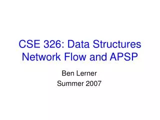
CSE 326: Data Structures Network Flow and APSP
CSE 326: Data Structures Network Flow and APSP. Ben Lerner Summer 2007. Network Flows. Given a weighted, directed graph G=(V,E) Treat the edge weights as capacities How much can we flow through the graph?. 1. F. 11. A. B. H. 7. 5. 3. 2. 6. 12. 9. 6. C. G. 11. 4. 10. 13.

CSE 326: Data Structures Network Flow and APSP
E N D
Presentation Transcript
CSE 326: Data StructuresNetwork Flow and APSP Ben Lerner Summer 2007
Network Flows • Given a weighted, directed graph G=(V,E) • Treat the edge weights as capacities • How much can we flow through the graph? 1 F 11 A B H 7 5 3 2 6 12 9 6 C G 11 4 10 13 20 I D E 4
Network flow: definitions • Define special source s and sink t vertices • Define a flow as a function on edges: • Capacity: f(v,w) <= c(v,w) • Skew symmetry: f(v,w) = -f(w,v) • Conservation: for all u except source, sink • Value of a flow: • Saturated edge: when f(v,w) = c(v,w)
Network flow: definitions • Capacity: you can’t overload an edge • Skew symmetry: sending f from uv implies you’re “sending -f”, or you could “return f” from vu • Conservation: Flow entering any vertex must equal flow leaving that vertex • We want to maximize the value of a flow, subject to the above constraints
Example (1) 2 3 4 1 2 4 2 2 Capacity
Example (2) 0/2 3/3 0/4 1/1 2/2 3/4 0/2 2/2 Flow / Capacity Are all the constraints satisfied?
Main idea: Ford-Fulkerson method • Start flow at 0 • “While there’s room for more flow, push more flow across the network!” • While there’s some path from s to t, none of whose edges are saturated • Push more flow along the path until some edge is saturated • Called an “augmenting path”
How do we know there’s still room? • Construct a residual graph: • Same vertices • Edge weights are the “leftover” capacity on the edges • Add extra edges for backwards-capacity too! • If there is a path st at all, then there is still room
Example (1) Initial graph – no flow 2 B C 3 4 1 A D 2 4 2 2 E F Flow / Capacity
Example (2) Include the residual capacities 0/2 B C 2 0/3 0/4 4 3 0/1 A D 2 1 0/2 0/4 2 0/2 4 0/2 E F 2 Flow / Capacity Residual Capacity
Example (3) Augment along ABFD by 1 unit (which saturates BF) 0/2 B C 2 1/3 0/4 4 2 1/1 A D 2 0 0/2 1/4 2 0/2 3 0/2 E F 2 Flow / Capacity Residual Capacity
Example (4) Augment along ABEFD (which saturates BE and EF) 0/2 B C 2 3/3 0/4 4 0 1/1 A D 0 0 2/2 3/4 2 0/2 1 2/2 E F 0 Flow / Capacity Residual Capacity
Now what? • There’s more capacity in the network… • …but there’s no more augmenting paths • But we broke our own rules – didn’t build the residual graph correctly
Example (5) Add the backwards edges, to show we can “undo” some flow 0/2 B C 3 2 3/3 0/4 4 1 0 A 1/1 D 0 0 2 2/2 3/4 2 0/2 1 2/2 E F 3 0 Flow / Capacity Residual Capacity Backwards flow 2
Example (6) Augment along AEBCD (which saturates AE and EB, and empties BE) 2/2 B C 3 0 2/4 3/3 2 1 0 A 1/1 D 0 2 2 0/2 3/4 0 2/2 1 2 E F 2/2 3 0 Flow / Capacity Residual Capacity Backwards flow 2
Example (7) Final, maximum flow 2/2 B C 2/4 3/3 A 1/1 D 0/2 3/4 2/2 E F 2/2 Flow / Capacity Residual Capacity Backwards flow
How should we pick paths? • Two very good heuristics (Edmonds-Karp): • Pick the largest-capacity path available • Otherwise, you’ll just come back to it later…so may as well pick it up now • Pick the shortest augmenting path available • For a good example why…
Bad example B 0/2000 0/2000 D A 0/1 C 0/2000 0/2000 Augment along ABCD, then ACBD, then ABCD, then ACBD… Should just augment along ACD, and ABD, and be finished
Running time? • Each augmenting path can’t get shorter…and it can’t always stay the same length • So we have at most O(E) augmenting paths to compute for each possible length, and there are only O(V) possible lengths. • Each path takes O(E) time to compute • Total time = O(E2V)
One more definition on flows • We can talk about the flow from a set of vertices to another set, instead of just from one vertex to another: • Should be clear that f(X,X) = 0 • So the only thing that counts is flow between the two sets
Network cuts • Intuitively, a cut separates a graph into two disconnected pieces • Formally, a cut is a pair of sets (S, T), such thatand S and T are connected subgraphs of G
Minimum cuts • If we cut G into (S, T), where S contains the source s and T contains the sink t, • What is the minimum flow f(S, T) possible?
Example (8) T S 2 B C 3 4 1 A D 2 4 2 2 E F Capacity of cut = 5
Coincidence? • NO! Max-flow always equals Min-cut • Why? • If there is a cut with capacity equal to the flow, then we have a maxflow: • We can’t have a flow that’s bigger than the capacity cutting the graph! So any cut puts a bound on the maxflow, and if we have an equality, then we must have a maximum flow. • If we have a maxflow, then there are no augmenting paths left • Or else we could augment the flow along that path, which would yield a higher total flow. • If there are no augmenting paths, we have a cut of capacity equal to the maxflow • Pick a cut (S,T) where S contains all vertices reachable in the residual graph from s, and T is everything else. Then every edge from S to T must be saturated (or else there would be a path in the residual graph). So c(S,T) = f(S,T) = f(s,t) = |f| and we’re done.
Single-Source Shortest Path • Given a graph G = (V, E) and a single distinguished vertex s, find the shortest weighted path from s to every other vertex in G. All-Pairs Shortest Path: • Find the shortest paths between all pairs of vertices in the graph. • How?
Analysis • Total running time for Dijkstra’s: O(|V| log |V| + |E| log |V|) (heaps) What if we want to find the shortest path from each point to ALL other points?
Dynamic Programming Algorithmic technique that systematically records the answers to sub-problems in a table and re-uses those recorded results (rather than re-computing them). Simple Example: Calculating the Nth Fibonacci number. Fib(N) = Fib(N-1) + Fib(N-2)
In section 10.3.4 in Weiss Can keep track of path with an extra matrix:path[i][j] = k if updating shortest path Floyd-Warshall Add in paths that go thru k for (int k = 1; k =< V; k++) for (int i = 1; i =< V; i++) for (int j = 1; j =< V; j++) if ( ( M[i][k]+ M[k][j] ) < M[i][j] ) M[i][j] = M[i][k]+ M[k][j] For iter k: will not be improving any paths that either start or finish at k(and these are the parts of the matrix you are examining to see if you found a new minimum, so the inner 2 loops could be executed in parallel.) Invariant: After the kth iteration, the matrix includes the shortest paths for all pairs of vertices (i,j) containing only vertices 1..k as intermediate vertices
Works with neg cost edges, but not neg cost cycles 2 b a -2 Initial state of the matrix: 1 -4 3 c 1 d e K=ano changesK=bM[ac] = M[a][b] + M[b][c] = 2 + -2 = inf to 0M[ae] = M[a][b] + M[b][e] = 2 + 3 = inf to 5K=cM[ae] = M[a][c] + M[c][e] = 0 + 1 = 5 to 1M[be] = M[b][c] + M[c][e] = -2 + 1 = 3 to -1K=dM[ae] = M[a][d] + M[d][e] = -4 + 4 = 1 to 0K=eno changes 4 M[i][j] = min(M[i][j], M[i][k]+ M[k][j])
2 b a -2 Floyd-Warshall - for All-pairs shortest path 1 -4 3 c 1 d e 4 Final Matrix Contents