Network Flow
Network Flow. Network flow. Use a graph to model material that flows through conduits. Each edge represents one conduit, and has a capacity, which is an upper bound on the flow rate = units/time. Can think of edges as pipes of different sizes.

Network Flow
E N D
Presentation Transcript
Network flow • Use a graph to model material that flows through conduits. • Each edge represents one conduit, and has a capacity, which is an upper bound on the flow rate = units/time. • Can think of edges as pipes of different sizes. • Want to compute max rate that we can ship material from a designated source to a designated sink.
Flow networks • G = (V, E) directed. • Each edge (u,v) has a capacity c(u, v) 0. • If (u, v) E, then c (u, v) = 0. • Source vertex s, sink vertex t, assume s v t for all v V. • Therefore, G is connected, and |E| |V| - 1
Flow • Let G be a flow network with a capacity function c. Let s be the source and t be the sink. • A flow in G is a real-valued function f : V V R satisfying • Capacity constraint : For all u, v V , f(u, v) ≤ c(u, v). • Skew symmetry : For all u, v V, f(u, v) = - f(v, u). • Flow conservation : For all u V – {s, t}, ∑ v Vf(u, v) = 0. • f(u, v) is called the flow from u to v, and can be positive, negative, or zero. • The value of a flow f is defined as | f | = ∑ v Vf(s, v) = total flow out of source. • Given a flow network G with capacity function c, source s and sink t, maximum-flow problem finds a flow of maximum value.
Positive flow • The total positive flow entering a vertex is defined by ∑ f (u, v). • The total positive flow leaving a vertex is defined symmetrically. • The total net flow at a vertex = total positive flow leaving a vertex – total positive flow entering a vertex. • Flow conservation says total positive flow entering a vertex (other than s or t ) = total positive flow leaving the vertex (“flow in = flow out”) v V f(u,v) > 0
Cancellation with flow • If we have edges (u, v) and (v, u), skew symmetry makes it so that at most one of these edges has positive flow. • Say f(u, v) = 5. If we “ship” 2 units v u, we lower f (u, v) to 3. The 2 units v u cancel 2 of the u v units. • Due to cancellation, a flow only gives us this “net” effect. We cannot reconstruct actual shipments from a flow. 5 units u v , 0 units v u is the same as 8 units u v , 3 units v u The flow from u to v remain f (u, v) = 5 and f (v, u) = -5.
Networks with multiple sources and sinks • If there are multiple sources {s1, s2 , …, sm } and sinks {t1, t2 , …, tn}, we can reduce the problem of determining a maximum flow in a network with multiple sources and multiple sinks to an ordinary maximum-flow problem. • We add a supersources and a directed edge (s, si) with capacity c(s, si) = for each i = 1, 2, …, m. • We add a supersinktand a directed edge (ti, t) with capacity c(ti, t) = for each i = 1, 2, …, n.
Implicit summation notation • Extend the notation of f, to take sets of vertices, with interpretation of summing over all vertices in the set. • If X and Y are sets of vertices, f (X, Y) = ∑∑ f (x, y). Therefore, can express flow conservation as f (u, V) = 0, for all u V – {s, t}. For convenience, omit set braces in the implicit summations. In equation f (s, V - s) = f (s, V ) , V – s means V – {s}. x X y Y
Lemma For any flow f in G = (V, E) : • For all X V, f (X, X ) = 0. • For all X, Y V, f (X, Y ) = - f (Y, X ). • For all X, Y, Z V with X ∩ Y = , f (X Y, Z ) = f (X, Z ) + f (Y, Z ) and f (Z, X Y ) = f (Z, X) + f (Z, Y )
Example Lemma : | f | = f (V, t). Pf)
Cuts • A cut (S, T ) of flow network G = (V, E ) is a partition of V into S and T = V – S such that s S and t T. • For flow f, the net flow across cut (S, T ) is f (S, T ). • Capacity of cut (S, T ) is c (S, T ). • A minimum cut of G is a cut whose capacity is minimum over all cuts of G.
Lemma • Lemma (26.5) For any cut (S, T ), f (S, T ) = | f | • Corollary (26.6) The value of any flow f in a flow network G ≤ capacity of any cut. • Therefore, maximum flow ≤ capacity of minimum cut. We’ll see later that maximum flow = capacity of minimum cut.
Residual network • Given a flow f in network G = (V, E ), consider a pair of vertices u, v V. How much additional flow can we push directly from u to v ? That’s the residual capacity, cf (u, v) = c (u, v) – f (u, v) 0 • Residual network: Gf (V, Ef ), Ef = { ( u, v ) V V : cf (u, v) > 0}. • Each edge of the residual network (residual edge ) can admit a positive flow. • The edges in Ef is either edges in E or their reversals. Thus, | Ef | ≤ 2 | E |
Residual network • Residual network Gf is itself a flow network with capacities given by cf • Given flows f 1and f 2 , the flow sum f 1+ f 2 is defined by ( f 1+ f 2 ) (u, v ) = f 1 (u, v ) + f 2 (u, v ) for all u, v V . • Lemma 26.2 Given flow network G, a flow f in G, the residual network Gf , let f 'be any flow in Gf . Then the flow sum f + f 'is a flow in G with value | f + f '| = | f | + | f ' | .
Augmenting path • Given a flow network G and a flow f, an augmenting path p is a simple path from s tot in the residual network Gf . • Each edge (u, v) on an augmenting path can admit some additional positive flow from u to v. • We call the maximum amount by which we can increase the flow on each edge in an augmenting path p, the residual capacity of p, given by cf (p) = min {cf (u, v): (u, v) is on p }.
Lemma 26.3. Let G = (V, E ) be a flow network, let f be a flow in G, let p be an augmenting path in Gf . .Define a function fp : V V R by fp (u, v) = cf (u, v)if (u, v) is on p, - cf (u, v)if (v, u) is on p 0 otherwise. Then fp is a flow in Gf with value | fp | = cf (p) > 0 Corollary Given flow network G, flow f in G, and an augmenting path p in Gf , define fpas in lemma, and define f’ : V V R by f’ = f + fp. Then f’ is a flow in G with value | f’ | = | f | + cf (p) > | f |.
Theorem 26.7 (Max-flow min-cut theorem) The following are equivalent : • f is a maximum flow. • f admits no augmenting path. • | f | = c(S,T ) for some cut (S,T ).
Ford-Fulkerson algorithm FORD-FULKERSON (G, s, t) for each edge (u,v) E(G) dof [u,v] ← f [v,u]← 0 while there is an augmenting path p in Gf docf (p) ← min {cf (u, v): (u, v) is on p } for each edge (u,v) in p dof [u,v] ← f [u,v] + cf (p) f [v,u] ← - f [u,v]
Analysis of Ford-Fulkerson • Running time depends on how the augmenting path is determined. (It may not even terminate for irrational capacities!) • If capacities are all integers, then each augmenting path raises | f | by ≥1. If max flow is f* , then need ≤ | f* | iterations. O(E | f* | ). • We can improve the bound if we implement the computation of the augmenting path p with a breadth-first search ( = if the augmenting path is a shortest path from s to t in the residual network with all edge weights = 1. ) This is called Edmonds-Karp algorithm.
Analysis of Edmonds-Karp algorithm • Edmonds-Karp runs in O(V E2) time. • To prove, need to look at distances to vertices in Gf • Let δf (u,v) = shortest path distance u to v in Gf with unit edge weights. • Lemma(26.8) : For all v V – {s, t} , δf (s,v) increases monotonically with each flow augmentation. • Theorem(26.9) : Edmonds-Karp performs O(V E ) augmentations. • Use BFS to find each augmenting path in O(E) time. • “push-relabel algorithms” can yield better bounds (O(V2E) in Section 26.4, O(V3) in Section 26.5)
Maximum bipartite matching • G = (V, E) (undirected ) is bipartite if we can partition V = L R such that all edges in E go between L and R. • A matching is a subset of edges M E such that for all v V , ≤ 1 edge of M is incident on v (vertex v is matched if an edge of M is incident on it; otherwise unmatched). • Maximum matching : a matching of maximum cardinality. • Problem : given a bipartite graph G = (V, E), find a maximum matching. • Define flow network G’ = (V’, E’), • V’ = V {s, t}. • E’ = {(s, u) : u L } { (u,v) : u L, v R} { (v,t) : v R}. • c(u,v)=1 for all (u,v) E’.
Lemma If M is a matching in G, then there is an integer-value flow f in G’ with value | f | = |M|. If f is an integer-valued flow in G’, then there is a matching M in G with cardinality |M| = | f | . • Integrality theorem : If the capacity function c takes only integral values, then the maximum flow f produced by the Ford-Fulkerson method has the property that |f | is integer-valued. Moreover, for all vertices u and v, the value of f (u,v) is an integer.
Push-relabel algorithms • Works on one vertex at a time, looking only at the vertex’s neighbors in the residual network. • Do not maintain flow conservation property throughout the execution. • Maintain a preflow f, which satisfies skew symmetry, capacity constraints, and f (V,u)≥ 0 for all vertices u V – {s}. • Excess flow into u is given by e(u) = f (V,u) • Vertex u V – {s, t} is overflowing if e(u) > 0.
Push-relabel algorithms • Each vertex has heights. Push flow downhill, from a higher vertex to a lower vertex. • The height of the source is |V |, and the height of the sink is fixed at 0. • All other vertex heights start at 0 and increase with time. • First, send as much flow as possible downhill from the source toward the sink – sends the capacity of the cut (s, V – s). • When the only pipes that leave a vertex u and are not already saturated with flow connect to vertices that are not downhill from u, increase its height (“relabel” u ) – increase the height to be one more than the height of the lowest of its neighbors to which it has an unsaturated pipe. • After all the flow that can get to the sink has arrived there, make the preflow a “legal” flow by sending the excess of overflowing vertices back to the source by relabeling vertices to above the fixed height |V| of the source.
Basic operations • Two basic operations : pushing flow excess from a vertex to one of its neighbors, and relabeling a vertex. • A function h : V → Nis a height function if h(s) = |V |, h(t) = 0, and h(u) ≤ h(v) + 1 for every residual edge (u, v) Ef. • Lemma 26.13 : Let G=(V, E) be a flow network, let f be a preflow in G, and let h be a height function on V. For any two vertices u, v V, if h(u) > h(v) + 1, then (u,v) is not an edge in the residual graph.
Push operation PUSH(u,v) Applies when : u is an overflowing , cf (u, v) > 0, and h(u) = h(v) + 1. Action : Push df (u, v) = min(e[u], cf (u, v)) from u to v. df (u, v) ← min(e[u], cf (u, v)) f [u, v] ← f [u, v] + df (u, v) f [v, u] ← - f [u, v] e[u] ← e[u] - df (u, v) e[v] ← e[v] + df (u, v) • If edge (u,v) becomes saturated (cf (u, v) = 0 afterward), it is a saturating push. Otherwise, a nonsaturating push. • Lemma : after a nonsaturating push from u to v, v is no longer overflowing.
Relabel operation RELABEL(u) Applies when : u is overflowing, and for all v V such that (u, v) Ef , h(u) ≤ h(v) . Action : increase the height of u. h(u) ← 1 + min{h(v) : (u, v) Ef } • After RELABEL(u), Ef contains at least one edge that leaves u because u is overflowing. So it gives u the greatest height allowed by the constraint on height functions,h(u) ≤ h(v) + 1 for every residual edge (u, v) Ef.
Initialization INITIALIZE-PREFLOW(G, s) for each vertex u V [G] do h[u]← 0 e[u]← 0 for each edge (u, v) E[G] do f [u, v] ← 0 f [v, u] ← 0 h[s]← | V [G] | for each vertex u Adj[s] do f [s, u] ← c(s, u) f [u, s] ← -c(s, u) e[u] ← c(s, u) e[s] ← e[s] - c(s, u)
Generic algorithm GENERIC-PUSH-RELABEL(G) INITIALIZE-PREFLOW(G,s) while there exists an applicable push or relabel operation do select an applicable push or relabel operation and perform it • Lemma : An overflowing vertex can be either pushed or relabeled.
Correctness of the push-relabel method • Prove that if it terminates, the preflow f is a maximum flow. • Prove that it terminates. • Lemma : Vertex heights never decrease during the execution of the algorithm. Whenever relabel operation is applied to u, h[u] increases by at least 1. • Lemma : During the execution of the algorithm, h is maintained as a height function. • Lemma : Let f be a preflow in a flow network G. Then, there is no path from s to t in the residual network Gf • Theorem : If the algorithm terminates, the preflow f compute is a maximum flow.
Analysis of the push-relabel method • Lemma : For any overflowing vertex u, there is a simple path from u to s in the residual network Gf . • Lemma : At any time during the execution of the algorithm, h[u] ≤ 2 |V | - 1 for all vertices u V. • Corollary : The number of relabel operations is at most h[u] ≤ 2 |V | - 1 per vertex and at most (2 |V | - 1 )(|V | - 2 ) < 2 |V |2overall. • Lemma : The number of saturating pushes is < 2 |V | | E |. • Lemma : The number of nonsaturating pushes is <4|V |2(|V |+ |E| ). • Theorem : the number of basic operations is O(V 2 E)
Relable-to-front algorithm • A push-relabel algorithm but choosing the order of basic operations carefully. • O(V 3) running time. • Maintains a list of the vertices in the network • Beginning at the front, scan the list repeatedly selecting an overflowing vertex u and then “discharging” it. (“discharge” = push and relabel until u is no longer overflowing.) • Whenever a vertex is relabeled, it is moved to the front of the list and the algorithm begins its scan anew.
Admissible edges and networks • If G=(V, E) be a flow network, f is a preflow in G, and h is a height function, then (u, v) is anadmissible edgeif cf (u, v) > 0, and h(u) = h(v) + 1. Otherwise, (u, v) is inadmissible. • The admissible network is Gf,h =(V, Ef,h ), whereEf,his the set of admissible edges. • The admissible network consists of those edges through which flow can be pushed. • Lemma : admissible netwosk is acyclic. • Lemma : if a vertex u is overflowing, and (u,v) is an admissible edge, then PUSH(u,v) applies. It does not create any new admissible edges, but it may make (u,v) inadmissible. • Lemma : if u is overflowing, and there is no admissible edges leaving u, RELABEL(u) applies. After operation, there is at least one admissible edge leaving u, but no admissible edges entering u.
Neighbor lists • Neighbor list N [u] for a vertex u V is a singly linked list of the neighbors of u in G. • head[N [u]] – points the first vertex in N [u] • next-neighbor[v] – points the next vertex in the list Relable-to-front algorithm cycles through each neighbor list in an arbitrary order fixed throughout the execution. For each vertex u, current[u] points to the vertex currently under consideration in N [u] Initially, current[u] is set to head[N [u]]
Discharging an overflowing vertex • An overflowing vertex u is discharged by pushing all its excess flow through admissible edges, relabeling u as necessary to cause edges leaving u to become admissible. DISCHARGE(u) while e[u] > 0 do v ← current[u] if v = NIL then RELABEL(u) current[u] ← head[N[u]] elsif cf (u, v) > 0, and h(u) = h(v) + 1 then PUSH(u,v) else current[u] ← next-neighbor[v]
Relable-to-front algorithm RELABLE-TO-FRONT(G,s,t) INITIALIZE-PREFLOW(G,s) L ← V[G] – {s, t}, in any order for each vertex u V[G] – {s,t} do current[u] ← head[N[u]] u ← head[L] while u NIL do old-height ← h[u] DISCHARGE(u) if h[u] > old-height then move u to the front of list L u ← next[u]
Correctness of relabel-to-front • An implementation of generic push-relabel algorithm – performs push and relabel operations only when they apply. • Need to show when relabel-to-front terminates, no basic operations apply. • Loop invariant : List L is a topological sort of the vertices in the admissible network and no vertex before u in the list has excess flow.