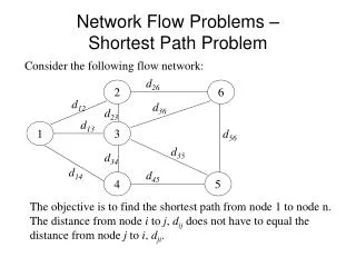
Network Flow Problems
Network Flow Problems. A special case of linear programming which is faster and has wide applicability. Solving Discrete Problems. Linear programming solves continuous problem — problems over the reaI numbers. For the remainder of the course we will look at how to solve

Network Flow Problems
E N D
Presentation Transcript
Network Flow Problems A special case of linear programming which is faster and has wide applicability
Solving Discrete Problems • Linear programming solves continuous problem • —problems over the reaI numbers. • For the remainder of the course we will look at how to solve • problems inwhich variables must take discrete values • —problems over the integers. • Discrete problems are harder than continuous problems. • We already saw: Finite Domain Propagation • We will look at • Network Flow Problems • Integer Programming • Boolean Satisfiability • Local Search
Network Simplex A particular form of linear integer problems can be solved in elegantly (and efficiently) with a drastic simplification of the simplex method d5=8 n1 d4=10 d3=6 n2 s6=9 s7=15 Network Flow Optimization
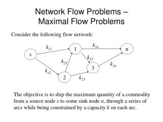
d5=8 n1 d4=10 d3=6 n2 s7=15 s6=9 Transshipment Problems • Intuitively, a transshipment problem (or network flow problem) • consists in finding the cheapest way of shipping goods through a • network of routes so that all given demands at all points of the • network are satisfied. Given: • a network of routes as a graph • a set of nodes which act as sources (supplies) • a set of nodes which act as sinks (demands) • the amount of supply and demand at each node • the cost of each transport route (edge) $29 $5 $18 $37 $8 $53 $28 $44 $59 $60 $98 $38 $23 $14 • Assumption: the total supply equals the total demand
Network Flow Matrix Representation A transshipment problem can concisely be represented in matrix form. with Incidence Matrix and Demand Vector. The incidence matrix A contains one column a=(a1, ..., an) for each edge e=(ni, nj) in the network with ak := -1 if k=i 1 if k=j 0 otherwise
Network Flow Matrix Representation the demand vector contains one element for each node giving the total demand at this node. Supplies are indicated as negative demands. The cost vector contains one entry for each edge e=(ni, nj) with the cost of shipping one unit along this edge.
Transshipment Formalization the transshipment problem can now be formalized as: such that A is an incidence matrix and Every problem that can be expressed in this form is a transshipment problem and can be solved by the network simplex algorithm.
Truncated Matrix Note that the equations expressed in are not independent. Since each of these equations is the sum of the remaining n-1 equations. We can therefore arbitrarily delete one of the equations from the matrices A and b obtaining A’ and b’. The truncated problem has the same solution as the original problem.
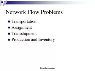
8 d5=8 n1 d4=10 1 9 9 d3=6 n2 6 15 s6=9 s7=15 Feasible Solutions = Trees Network Feasible Tree Solution Note that the feasible tree need not be a directed tree. It is defined on underlying undirected graph. If a transhipment problem has an optimal solution then it has an optimal solution that corresponds to a feasible tree solution. Why? Thus we need only consider feasible tree solutions.
d5=8 n1 d4=10 d3=6 n2 s6=9 s7=15 Uniqueness of Feasible Solutions For a given tree there is a unique assignment to the edges in the tree that satisfies the supply and demand constraints. This can be found using a recursive tree traversal. What is the assignment for this tree?
8 1 9 9 6 15 d5=8 n1 d4=10 d3=6 n2 s7=15 s6=9 Network Simplex $29 $5 $18 $37 $8 $53 $28 $44 $59 $60 $98 $38 $23 $14 Network Feasible Spanning Tree Solution The Network Simplex works by improving the current feasible spanning tree solution. Find an initial feasible tree solution While current solution not optimal Choose the edge to enter (choose new basic variable) Choose the edge to leave so it remains a tree (choose variable to leave) This exactly corresponds to the Simplex method but is greatly simplified because of the form of the constraints.
d5=8 n1 d4=10 d3=6 n2 s7=15 s6=9 Choosing the Edge to Enter $29 $29 $5 $18 $18 $37 $8 $53 $28 $44 $28 $59 $59 $44 $60 $60 $98 $38 $23 $23 $14 For each edge not in the spanning tree work out the benefit (gain) of adding it and moving 1 unit along that edge. In the case of the edge (n7,n5) the cost of moving 1 unit along the edge is 1*59-1*29+1*18-1*28-1*23 = -3. So the benefit is 3 and we will reduce the cost if we add this edge. If no edge has a benefit > 0 then the solution is optimal. Otherwise choose some edge with positive benefit to add.
Computing the Edge Benefit $29 Y5= Y1= We can compute the edge benefit more efficiently than this by thinking about the Simplex. (See Winston Chap 8 for justification). $18 Y4= $28 $59 $44 Y2= Y3= $60 $23 Y7=0 Y6= In the Simplex we compute the opportunity cost for each resource. The benefit we have just computed is exactly the opportunity cost for the edge. For each node ni we associate a variable yi which is (sort of) the price of shipping 1 unit to that node from an arbitrary origin node. This is the negative of the Simplex multiplier. If an edge (ni,nj) is in the tree then yj=yi+cij. This allows us to easily compute the yi’s. (We assume that for the origin node yi =0) The opportunity cost cij for an edge (ni,nj) not in the tree is cij=yj-yi-cij.
Entering Edges An edge with positive benefit is now added to the spanning tree. It is therefore called the “entering edge”. Strategy: If there are several possible choices for entering edges, choose the one with maximum benefit. Note: large scale computer implementations use different strategies
8 1 9 9 6 15 Network Pivot The pivot step improves the solution by shipping some quantity t along the entering edge. As in the Simplex we try to exploit the entering edge maximally by maximizing t until constraints are tight. The obvious adjustments are obtained by traversing the cycle introduced by the entering edge (in its direction) and labelling each edge a along the cycle with (xij+t) if a has the same direction on the cycle as the entering edge (xij-t) if a has the opposite direction on the cycle. With the resulting adjustments we have to satisfy: t ≥ 0, 8-t ≥ 0, 9-t ≥ 0, 15-t ≥ 0, 1+t ≥ 0 This leads to t=8 which removes all shipments from the dotted edge. This edge is referred to as the “leaving edge”. 8-t 1+t 9-t t units 9 6 15-t 9 1 8 9 6 7
Summary: Network Simplex (1) construct a basic feasible tree. (2) compute the benefit for each edge for this tree. (3a) find an entering edge that can improve the solution (3b) if no such edge can be found, the solution is optimal (4) adjust the quantities shipped (5) re-iterate from step (2) As the Simplex algorithm, network simplex only works with feasible solutions. The obvious problem is how to find an initial basic feasible tree!
Basic Feasible Tree Construction In general, finding a basic feasible tree is not simple. However, we can perform a “trick” similar to Simplex phase 0. The basic idea is to add “artificial arcs” that guarantee a trivial basic feasible tree. We then use a phase 0 optimization on the augmented graph that penalizes these arcs so that they are not used in the optimum solution to phase 0. The result of phase 0 with the (unused) artificial arcs removed is then a basic feasible solution for the original problem.
Auxiliary Problem & Graph • Select an arbitrary fixed node w • Add an artificial edge from w to each node • set xwj=bj • The set of artificial edges forms a feasible spanning tree for the auxiliary graph • Solve the following auxiliary problem • set penalty pij=1 for each artificial edge • set penalty pij=0 for each original edge
Solving the Auxiliary Problem • The auxiliary problem can simply be optimized by network simplex. • Three outcomes for the spanning tree T of the solution of phase 0 • are possible: • T contains no artificial edge -> use T as a start for phase I optimization of original problem • T contains an artificial edge aij with xij>0 -> the original problem is infeasible • T contains artificial arcs aij with xij=0 -> the original problem may have a solution, but not a tree solution (eg network not sufficiently connected) • Decompose the original problem into two networks. Let a=(ni, nj) be the artificial edge with xij=0 • - Network A contains all nodes that precede ni in T • - Network B contains all nodes that follow ni in T • A and B can now be solved independently
Integrality Theorem • Let b be a vector of integers. • The transshipment problem • (a) is feasible if and only if • it has an integer-valued solution vector x. • (b) has an optimal solution if and only if • it has an integer-valued optimal solution. • This can be proved by analyzing the pivot operation of the network simplex: • Whenever it starts from an integer-valued solution the subsequent • solution is also integer-valued.
Complexity • Linear Programming: • Interior point methods • worst case: polynomial • Simplex algorithm • worst case: exponential in size of LP • in practice: well-behaved • Integer Linear Programming: NP-complete • Network Simplex • worst case: exponential in node size • (proven for largest merit selection ‘73) • in practice: roughly linear in node size • However, there are versions of Network Simplex with • polynomial worst case behaviour (proved in 1997!)
Generalization to Inequalities (supply matches demand) is often unrealistic The assumption • We need to generalize to supplies that exceed the demand. • Introduce “virtual dump” (new node) for exceeding supply d5=8 n1 d4=10 d3=6 n2 s7=15+y s6=9+x dvd=x+y The new “dummy node” must be connected to each source by a new “dummy edge” of zero cost.
Caterer Problem (aircraft overhaul scheduling) • A caterer needs to plan (and optimize) his napkin provisions over n days • dj: number of napkins needed on day j (known in advance) • Napkins can be • bought: a cents per piece • laundered: • b cents per napkin (fast service takes q days) • c cents per piece (slow service takes p days) +d1 “q days” “buy” “quick laundry” -d1 “p days” Shop “keep” “slow” exceeding supply in shop +dn -dn Dump “at end of day” “at start of day”
Summary • We have looked at • Transhipment problems (network flow) • Network simplex • Gives an efficient way of solving some IP problems • Can be generalized to handle an upper bound on the flow along an edge Homework • Read Winston Chap 8 • Solve the example using network simplex • Do the assignment!