Deep-water “limiting” envelope solitons
370 likes | 539 Vues
Deep-water “limiting” envelope solitons. Alexey Slunyaev. Institute of Applied Physics RAS, Nizhny Novgorod. Motivation. NLS envelope solitons. two collision of solitons. ka = 0.085. [Zakharov et al, 2006]. Limiting envelope solitons.

Deep-water “limiting” envelope solitons
E N D
Presentation Transcript
Deep-water “limiting” envelope solitons Alexey Slunyaev Institute of Applied Physics RAS, Nizhny Novgorod
NLS envelope solitons two collision of solitons ka = 0.085 [Zakharov et al, 2006]
Limiting envelope solitons appearance and propagation of “limiting” envelope solitons (“breathers”) steepness profile [Dyachenko & Zakharov, 2008]
? How do the approximate (high-order) envelope eqs and fully nonlinear description of steep envelope solitary waves relate?
Brief overview of the history Water wave envelope solitons Envelope solitons results from modulational instability (~1965) Envelope solitons are the asymptotic solution of NLS (1968, 1971, 1973) Collision of envelope solitary waves Longuet-Higgins & Phillips, JFM 1962 (analytics) Feir, Proc R Soc A 1965 (experiment) Zakharov & Shabat, JETP 1971, 1973 (integrability) Dommermuth & Yue, JFM 1987 (HOSM) West et al, JGR 1987 (HOSM) Zakharov et al, Eur J Mech B Fl 2006 (full eds)
Full numerical model incompressible inviscid irrotational water potential movement gravity force infinite depth periodic boundary conditions Euler eqs in conformal variables [Zakharov et al, 2002] High-Order Spectral Method (HOSM), M = 6 [Dommermuth&Yue, West et al, 1987]
Choosing the approximate model Modulation equations Classic NLS Soliton solution NLS-2 Dysthe or MNLS
Approximate model , Free and bound waves Example of a laboratory frequency spectrum of intense narrow-banded wave groups . Bound wave 3 order corrections
Single envelope solitons Initial condition Exact solution of the NLS soliton Bound wave correction
Single envelope solitons Initial condition Nonlinearity / dispersion ration in the NLS eq «Nonlinear» time
Propagation of single solitons Surface displacements ka = 0.2, T0 = 2 Tnl 50 Full Dysthe ka = 0.3, T0 = 2 Tnl 20 Full Dysthe
Propagation of single solitons Characteristic steepness & max wave slope k [max((x)) – min((x))] / 2 max|x| ka = 0.2, T0 = 2 Tnl 50 Full Dysthe ka = 0.3, T0 = 2 Tnl 20 Full Dysthe
Propagation of single solitons Role of high-order corrections Accuracy Model Eq Field reconstruction Soliton solution Classic NLS O(3) 1 O(3) Dysthe O(3+1) 1 + 2 O(3+1) We use O(3+1) 1 + 2 +3 O(3)
Propagation of single solitons Role of high-order corrections ka = 0.3, T0 = 2 3-order bound wave corrections Full Dysthe no bound wave corrections Full Dysthe
Soliton interaction Toward propagation a1 = 0.2, a2 = 0.2k1 = 1, k2 = 1k1a1 = 0.2, k2a2 = 0.2 a1 = 0.2, a2 = 0.1k1 = 1, k2 = 1k1a1 = 0.2, k2a2 = 0.1 a1 = 0.2, a2 = 0.1k1 = 1, k2 = 2k1a1 = 0.2, k2a2 = 0.2
Soliton interaction Toward propagation half-height & slope
Soliton interaction Toward propagation after 7 (6) collisions
Soliton interaction Comoving propagation a1 = 0.1, a2 = 0.1k1 = 1, k2 = 2k1a1 = 0.1, k2a2 = 0.2 a1 = 0.05, a2 = 0.1k1 = 1, k2 = 2k1a1 = 0.05, k2a2 = 0.2 a1 = 0.2, a2 = 0.1k1 = 1, k2 = 2k1a1 = 0.2, k2a2 = 0.2
Soliton interaction Comoving propagation half-height & slope
Soliton interaction Comoving propagation after one collision
Soliton interaction Bi-soliton Exact 2-soliton solution of NLS + bound wave corrections a1 = 0.2, a2 = 0.1 k = 1ka1 = 0.1, ka2 = 0.2
Soliton interaction Bi-soliton Full Tnl 50 Dysthe
Soliton interaction Bi-soliton Coupled nonlinear groups Full a1 = 0.08, a2 = 0.04 k = 1ka1 = 0.08, ka2 = 0.04 Dysthe overlapping solitons & not exact solution 100Tnl background noise long-time simulation non-Hamiltonian Dysthe eq 400Tnl
Conclusions Existence of “limiting” envelope solitons has been shown [Dyachenko & Zakharov, 2008] High-order envelope models describe the “limiting” envelope solitons (up to ka~ 0.2...0.3) quite well Occasional wave steepening seems to be the only reason why the “limiting” envelope solitons are difficult to reproduce Toward-propagating envelope solitons collide in a great extent elastically When co-moving solitons interact, a higher and longer-wavelength soliton destroys the smaller and shorter-wavelength one Long-time interacting solitons (with similar wavenumbers) can couple