Analysis of Variance - ANOVA
370 likes | 1.67k Vues
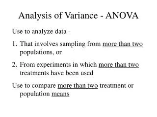
Analysis of Variance - ANOVA. Use to analyze data - That involves sampling from more than two populations, or From experiments in which more than two treatments have been used Use to compare more than two treatment or population means. Definitions.

Analysis of Variance - ANOVA
E N D
Presentation Transcript
Analysis of Variance - ANOVA • Use to analyze data - • That involves sampling from more than two populations, or • From experiments in which more than two treatments have been used • Use to compare more than two treatment or population means
Definitions Factor – The characteristic that distinguishes the treatments or populations from one another Levels – This refers to the different treatments or populations Single-Factor ANOVA (chapter 10) Multi-Factor ANOVA (chapter 11)
Example • An experiment to study the effects of four different brands of gasoline (Exxon, Conoco, Shell, Texaco) on the fuel efficiency (mpg) of a car • Factor – Gasoline Brand • Levels – the 4 brands (Exxon, Conoco, Shell, Texaco) • Single-Factor ANOVA
Example • An experiment to study the effects of four different brands (Exxon, Conoco, Shell, Texaco) and three different types of gasoline (regular, midgrade, premium) on the fuel efficiency (mpg) of a car • Factor – Gasoline Brand, Gasoline Type • Levels – the 4 brands (Exxon, Conoco, Shell, Texaco), the 3 types (Regular, midgrade, premium) • Two-Factor ANOVA
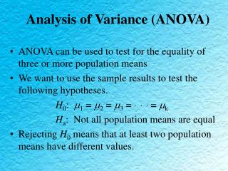
Mathematical Specification I = Number of Populations or Treatments being Compared The mean of population i or the true average when treatment i is applied The hypotheses of interest are: Ho:1= 2 = …… = i Ha: at least two of the i’s are different
Single-Factor ANOVA J = Number of observations in each sample; Assume each sample has same # observations Xi,j = jth measurement from the ith population or treatment A dot indicates that we have summed over that subscript
Single-Factor Cont’d Individual Sample Means:
Single-Factor Cont’d Grand Mean:
Assumptions • The I population or treatment distributions are Normal • Each of these distributions has the same variance, i.e. 12 = 22 = …. = n2
Development of Test Statistic MSTr describes “between-samples” variation MSE describes “within-samples” variation
Computational Formulas Cont’d Identity: SST = SSTr + SSE • Partition total variation into two pieces • SSE (within) measures variation that would be present even if Ho true (unexplained by Ho when true or false) • SSTr (between) measures amount of variation that can be explained by possible differences in the i’s (explained by Ho when false)
Example Our manufacturing firm in interested in the concentration of impurities in steel obtained from four different vendors. Test the hypothesis that the mean concentration of impurities is the same for all vendors at a 0.01 level of significance.
Example Data – I=4, J=10 Vendor 1: 20.5, 28.1, 27.8, 27.0, 28.0, 25.2, 25.3, 20.5, 31.3 Vendor 2: 26.3, 24.0, 26.2, 20.2, 23.7, 34.0, 17.1, 26.8, 23.7, 24.9 Vendor 3: 29.5, 34.0, 27.5, 29.4, 27.9, 26.2, 29.9, 29.5, 30.0, 35.6 Vendor 4: 36.5, 44.2, 34.1, 30.3, 31.4, 33.1, 34.1, 32.9, 36.3, 25.5