Markov Model
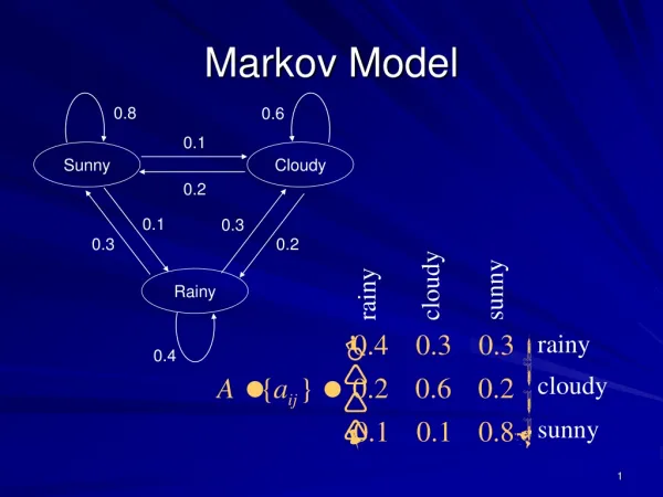
Markov Model. 0.8. 0.6. 0.1. Sunny. Cloudy. 0.2. 0.1. 0.3. 0.3. 0.2. cloudy. sunny. Rainy. rainy. rainy. 0.4. cloudy. sunny. Markov Model ( Con’d ). Discrete Markov Model. Degree 1 Markov Model. Markov Model Example. How much is this probability:

Markov Model
E N D
Presentation Transcript
Markov Model 0.8 0.6 0.1 Sunny Cloudy 0.2 0.1 0.3 0.3 0.2 cloudy sunny Rainy rainy rainy 0.4 cloudy sunny
Markov Model (Con’d) • Discrete Markov Model Degree 1 Markov Model
Markov Model Example • How much is this probability: • Sunny, Sunny, Sunny, Rainy, Rainy, Sunny, Cloudy, Cloudy
Markov Model Example (Cont’d) • The probability of being in state in time • The probability of staying in state for days if we are in state ? d Days
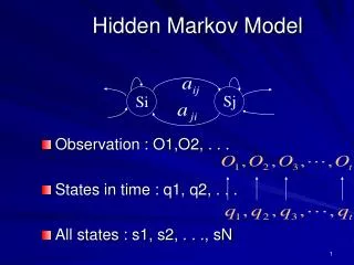
Hidden Markov Model • If you don’t have complete state information, but some observations at each state N: Number of states states = M: Number of observationsobservations =
Hidden Markov Model 0.8 0.6 0.1 Sunny Cloudy 0.2 Umbrella?Y: 0.1 N: 0.9 0.1 Umbrella?Y: 0.3 N: 0.7 0.3 0.3 0.2 Seeing your colleague with an umbrella Seeing your colleague without an umbrella Rainy Umbrella?Y: 0.8 N: 0.2 0.4 rainy cloudy sunny
Discrete Density HMM Components • N: Number Of States • M: Number Of Outputs • A (NxN): State Transition Probability Matrix • B (NxM): Output Occurrence Probability in each state • (1xN): Initial State Probability : Set of HMM Parameters
Three Basic HMM Problems • Recognition Problem: Given an HMM and a sequence of observations O,what is the probability ? • State Decoding Problem: Given a model and a sequence of observations O, what is the most likely state sequence in the model that produced the observations? • Training Problem: Given a model and a sequence of observations O, how should we adjust model parameters in order to maximize ?
First Problem Solution We Know That: And
First Problem Solution (Cont’d) Computation Order :
Forward Backward Approach Computing 1) Initialization
Forward Backward Approach (Cont’d) 2) Induction : 3) Termination : Computation Order :
Backward Variable 1) Initialization 2)Induction
Second Problem Solution • Finding the most likely state sequence Individually most likely state :
Viterbi Algorithm • Define : P is the most likely state sequence with this conditions : state i , time t and observation o
Viterbi Algorithm (Cont’d) 1) Initialization Is the most likely state before state i at time t-1
Viterbi Algorithm (Cont’d) 2) Recursion
Viterbi Algorithm (Cont’d) 3) Termination: 4)Backtracking:
Third Problem Solution • Parameters Estimation using Baum-Welch Or Expectation Maximization (EM) Approach Define:
Third Problem Solution (Cont’d) : Expected value of the number of jumps from state i : Expected value of the number of jumps from state i to state j
Baum Auxiliary Function By this approach we will reach to a local optimum
Continuous Observation Density • We have amounts of a PDF instead of • We have Mixture Coefficients Variance Average
Continuous Observation Density • Mixture in HMM M1|1 M1|2 M1|3 M2|1 M2|2 M2|3 M3|1 M3|2 M3|3 M4|1 M4|2 M4|3 S2 S3 S1 Dominant Mixture:
Continuous Observation Density (Cont’d) • Model Parameters: N×M×K×K 1×N N×M N×M×K N×N N : Number Of States M : Number Of Mixtures In Each State K : Dimension Of Observation Vector
Continuous Observation Density (Cont’d) Probability of event j’th state and k’th mixture at time t
State Duration Modeling Sj Si Probability of staying d times in state i :
State Duration Modeling (Cont’d) HMM With clear duration ……. ……. Sj Si
State Duration Modeling (Cont’d) • HMM consideration with State Duration : • Selecting using ‘s • Selecting using • Selecting Observation Sequence using in practice we assume the following independence: • Selecting next state using transition probabilities . We also have an additional constraint:
Training In HMM • Maximum Likelihood (ML) • Maximum Mutual Information (MMI) • Minimum Discrimination Information (MDI)
Training In HMM • Maximum Likelihood (ML) . . . Observation Sequence
Training In HMM (Cont’d) • Maximum Mutual Information (MMI) Mutual Information
Training In HMM (Cont’d) • Minimum Discrimination Information (MDI) Observation : Auto correlation :
Typical HMM Models • Ergodic Model: • Left-to-right Model:
Left-to-right Model Parameters • If we want to control large changes in states:
Autoregressive HMM • The observation Otcomes from a distribution that is determined by the current state of the process qt. (or possibly past observations and past states). • The distribution of Otis normal with mean and variance
Autoregressive HMM (Cont’d) • Additional Model Parameters • State Means • State Variances • State Autoregressive Parameters
Null Transition • Transitions which produce no output, and take no time, denoted by φ • For example to model alternate word pronunciations (look at 2 possible different “two”s)
State Tying • A parameter is said to be tied in the HMMs of two sound units if it is identical for both of them • E.g. if transition probabilities are assumed to be identical for both, the transition probabilities for both are “tied” • useful in cases where there is insufficient training data for reliable estimation of all model parameters • number of independent parameters of the model reduced • State-tying is a form of parameter sharing where the state output distributions of different HMMs are the same • All state-of-art speech recognition systems employ state-tying at some level or the other • The most common technique uses decision trees
Is right contextan affricate? yes no Is left contexta vowel? Is left contexta glide? yes no yes no Group 1 Group 2 Group 3 Is right contexta glide? yes no Group 4 Group 5 State Tying (Cont’d) • A sample decision tree
Issues with HMM implementation • Scaling • Product of very small terms -> machine may not be precise enough, so we scale • Multiple observation sequences • In left-to-right model, small number of observations available for each state, requiring several sequences for parameter estimation (3rd Problem) • Initial estimate • Normal distributions fine for P ,A , but B is sensitive to initial estimate • Again, this is an issue for problem 3
Issues with HMM implementation (Cont’d) • Insufficient training data • For ex: not enough occurrences of different events in a given state • Possible solution: reduce model to subset for which more data exists, and linearly interpolate between model parameters • Alternately, could impose some lower bound on individual observation probabilities • Model choice • Ergodicvs. LTR (or other), Continuous vs. discrete observation densities, number of states, etc.
Overall Recognition System Word Dictionary (In Terms of Chosen Units) Grammar Task Model Inventory of Speech Recognition Units Recognized Speech Syntactic Analysis Semantic Analysis Lexical Decoding FeatureAnalysis Unit Matching System Utterance

