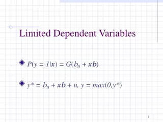
Models with limited dependent variables

1. Models with limited dependent variables Doctoral Program 2006-2007 Katia Campo

2. Introduction

3. Discrete Choice Models Truncated/ Censored Regr.Models Duration (Hazard) Models Limited dependent variables Discrete dependent variable Continuous dependent variable Truncated, Censored

4. Discrete choice models • Choice between different options (j) • Single Choice (binary choice models) e.g. Buy a product or not, follow higher education or not, ... • j=1 (yes/accept) or 0 (no/reject) • Multiple Choice (multinomial choice models), e.g. cars, stores, transportation modes • j=1(opt.1), 2(opt.2), ....., J(opt.J)

5. Truncated/censored regression models • Truncated variable: observed only beyond a certain threshold level (‘truncation point’) e.g. store expenditures, income • Censored variables: values in a certain range are all transformed to (or reported as) a single value (Greene, p.761) e.g. demand (stockouts, unfullfilled demand), hours worked

6. Duration/Hazard models • Time between two events, e.g. • Time between two purchases • Time until a consumer becomes inactive/cancels a subscription • Time until a consumer responds to direct mail/ a questionnaire • ...

7. Need to use adjusted models: Illustration Frances and Paap (2001)

8. Overview • Part I. Discrete Choice Models • Part II. Censored and Truncated Regression Models • Part III. Duration Models

9. Recommended Literature • Kenneth Train, Discrete Choice Methods with Simulation, Cambridge University Press, 2003 (Part I) • Ph.H.Franses and R.Paap, Quantitative Models in Market Research, Cambridge University Press, 2001 (Part I-II-III; Data: www.few.eur.nl/few/people/paap) • D.A.Hensher, J.M.Rose and W.H.Greene, Applied Choice Analysis, Cambridge University Press, 2005 (Part I)

10. Part I. Discrete Choice Models

11. Overview Part I, DCM • Properties of DCM • Estimation of DCM • Types of Discrete Choice Models • Binary Logit Model • Multinomial Logit Model • Nested logit model • Probit Model • Ordered Logit Model • Heterogeneity

12. Notation • n = decision maker • i,j = choice options • y = decision outcome • x = explanatory variables •  = parameters •  = error term • I[.] = indicator function, equal to 1 if expression within brackets is true, 0 otherwise e.g. I[y=j|x] = 1 if j was selected (given x), equal to 0 otherwise

13. A. Properties of DCM Kenneth Train • Characteristics of the choice set • Alternatives must be mutually exclusive no combination of choice alternatives (e.g. different brands, combination of diff. transportation modes) • Choice set must be exhaustive i.e., include all relevant alternatives • Finite number of alternatives

14. A. Properties of DCM Kenneth Train • Random utility maximization Ass: decision maker selects the alternative that provides the highest utility, i.e. Selects i if Uni > Unj j  i Decomposition of utility into a deterministic (observed) and random (unobserved) part Unj = Vnj + nj

15. A. Properties of DCM Kenneth Train • Random utility maximization

16. A. Properties of DCM Kenneth Train • Identification problems • Only differences in utility matter Choice probabilities do not change when a constant is added to each alternative’s utility • Implication Some parameters cannot be identified/estimatedAlternative-specific constants; Coefficients of variables that change over decision makers but not over alternatives Normalization of parameter(s)

17. A. Properties of DCM Kenneth Train • Identification problems • Overall scale of utility is irrelevant Choice probabilities do not change when the utility of all alternatives are multiplied by the same factor • Implication Coefficients of  models (data sets) are not directly comparable Normalization (var.of error terms)

18. A. Properties of DCM Kenneth Train • Aggregation Biased estimates when aggregate values of the explanatory variables are used as input Consistent estimates can be obtained by sample enumeration - compute prob./elasticity for each dec.maker - compute (weighted) average of these values Swait and Louvière(1993), Andrews and Currim (2002)

19. Properties of DCM Keneth Train • Aggregation

20. B. Estimation DCM • Numerical maximization (ML-estimation) • Simulation-assisted estimation • Bayesian estimation (see Train)

21. B. ML-estimation • Objective: “find those parameter values most likely to have produced the sample observations” (Judge et al.) • Likelihood for one observation: Pn(X,) • Likelihoodfunction L() = nPn(X,) • Loglikelihood LL() =  n ln(Pn(X,))

22. B. ML Estimation Determine for which LL() reaches its max • First derivative = 0  no closed-form solution • Iterative procedure: • Starting values 0 • Determine new value t+1 for which LL(t+1) > LL(t) • Repeat procedure ii until convergence (small change in LL())

23. B. ML Estimation

24. B. ML Estimation - Direction and step size t → t+1 ? based on taylor approximation of LL(t+1) (with base (t)) LL(t+1) = LL(t)+(t+1- t)’gt+1/2(t+1- t)’Ht (t+1- t) [1] with

25. B. ML Estimation - Direction and step size t → t+1 ? Optimization of [1] leads to:  Computation of the Hessian may cause problems

26. B. ML Estimation Alternatives procedures: • Approximations to the Hessian • Other procedures, such as steepest-ascent See e.g. Train, Judge et al.(1985)

27. B. ML Estimation Properties ML estimator Consistency Asymptotic Normality Asymptotic Efficiency See e.g. Greene (ch.17), Judge et al.

28. B.Diagnostics and Model Selection • Goodness-of-Fit • Joint significance of explanatory var’s LR-test : LR = -2(LL(0) - LL()) LR ~ ²(k) • Pseudo R² = 1 - LL() LL(0)

29. B.Diagnostics and Model Selection • Goodness-of-Fit • Akaike Information Criterion AIC = 1/N (-2LL() +2k) • CAIC = -2LL() + k(log(N)+1) • BIC = 1/N (-2LL() + k log(N)) • sometimes conflicting results

30. B.Diagnostics and Model Selection • Model selection based on GoF • Nested models : LR-test LR = -2(LL(r) - LL(ur)) r=restricted model; ur=unrestricted (full) model LR ~ ²(k) (k=difference in # of parameters) • Non-nested models AIC, CAIC, BIC  lowest value

31. C. Discrete Choice Models • Binary Logit Model • Multinomial Logit Model • Nested logit model • Probit Model • Ordered Logit Model

32. 1. Binary Logit Model • Choice between 2 alternatives • Often ‘accept/reject’ or ‘yes/no’ decisions • E.g. Purchase incidence: make a purchase in the category or not • Dep. var. yn = 1, if option is selected = 0, if option is not selected • Model: P(yn=1| xn)

33. 1. Binary Logit Model • Based on the general RUM-model • Ass.: error terms are iid and follow an extreme value or Gumbel distribution

34. 1. Binary Logit Model • Based on the general RUM-model • Pn =  I[β’xn + εn > 0] f(ε) dε =  I[εn > -β’xn] f(ε) dε = ε=-β’x f(ε) dε = 1 – F(- β’xn) = 1 – 1/(1+exp(β’xn)) = exp(β’xn)/(1+exp(β’xn)) Ass.: error terms are iid and follow an extreme value/Gumbel distr.

35. 1. Binary Logit Model • Leads to the following expression for the logit choice probability

36. 1. Binary Logit Model Properties • Nonlinear effect of explanatory var’s on dependent variable • Logistic curve with inflection point at P=0.5

37. 1. Binary Logit Model

38. 1. Binary Logit Model Effect of explanatory variables ? For Quasi-elasticity

39. 1. Binary Logit Model Effect of explanatory variables ? For Odds ratio is equal to

40. 1. Binary Logit Model Estimation: ML • Likelihoodfunction L() = nP(yn=1|x,)yn (1- P(yn=1|x,))1-yn • Loglikelihood LL() =  n yn ln(P(yn=1|x,) )+ (1-yn) ln(1- P(yn=1|x,))

41. 1. Binary Logit Model • Forecasting accuracy • Predictions : yn=1 if F(Xn ) > c (e.g. 0.5) yn=0 if F(Xn )  c • Compute hit rate = % of correct predictions

42. 1. Binary Logit Model Example: Purchase Incidence Model ptn(inc) = probability that household n engages in a category purchase in the store on purchase occasion t, Wtn = the utility of the purchase option. Bucklin and Gupta (1992)

43. 1. Binary Logit Model Example: Purchase Incidence Model With CRn = rate of consumption for household n INVnt = inventory level for household n, time t CVnt= category value for household n, time t Bucklin and Gupta (1992)

44. 1. Binary Logit Model • Data • A.C.Nielsen scanner panel data • 117 weeks: 65 for initialization, 52 for estimation • 565 households: 300 selected randomly for estimation, remaining hh = holdout sample for validation • Data set for estimation: 30.966 shopping trips, 2275 purchases in the category (liquid laundry detergent) • Estimation limited to the 7 top-selling brands (80% of category purchases), representing 28 brand-size combinations (= level of analysis for the choice model) Bucklin and Gupta (1992)

45. 1. Binary Logit Model Goodness-of-Fit

46. 1. Binary Logit Model Parameter estimates

47. Variable Coefficient Std. Error z-Statistic Prob. C 0.222121 0.668483 0.332277 0.7397 DISPLHEINZ 0.573389 0.239492 2.394186 0.0167 DISPLHUNTS -0.557648 0.247440 -2.253674 0.0242 FEATHEINZ 0.505656 0.313898 1.610896 0.1072 FEATHUNTS -1.055859 0.349108 -3.024445 0.0025 FEATDISPLHEINZ 0.428319 0.438248 0.977344 0.3284 FEATDISPLHUNTS -1.843528 0.468883 -3.931748 0.0001 PRICEHEINZ -135.1312 10.34643 -13.06066 0.0000 PRICEHUNTS 222.6957 19.06951 11.67810 0.0000 Binary Logit Model (Franses and Paap: www.few.eur.nl/few/people/paap)

48. Binary Logit Model (Franses and Paap: www.few.eur.nl/few/people/paap) Mean dependent var 0.890279 S.D. dependent var 0.312598 S.E. of regression 0.271955 Akaike info criterion 0.504027 Sum squared resid 206.2728 Schwarz criterion 0.523123 Log likelihood -696.1344Hannan-Quinn criter. 0.510921 Restr. log likelihood -967.918Avg. log likelihood -0.248797 LR statistic (8 df) 543.5673 McFadden R-squared 0.280792 Probability(LR stat) 0.000000 Obs with Dep=0 307 Total obs 2798 Obs with Dep=1 2491

49. Binary Logit Model (Franses and Paap: www.few.eur.nl/few/people/paap)

50. Binary Logit Model (Franses and Paap: www.few.eur.nl/few/people/paap)