Connecting atmospheric composition with climate variability and change
320 likes | 493 Vues
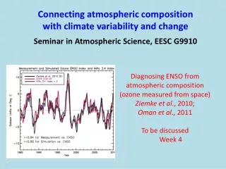
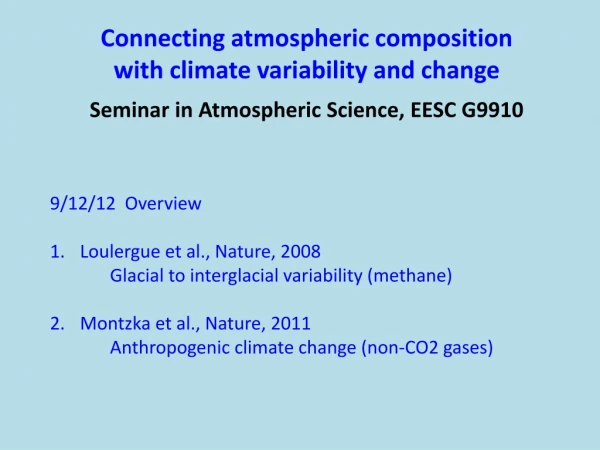
Connecting atmospheric composition with climate variability and change Seminar in Atmospheric Science, EESC G9910. 9/12/12 Overview Loulergue et al., Nature, 2008 Glacial to interglacial variability (methane) Montzka et al., Nature, 2011

Connecting atmospheric composition with climate variability and change
E N D
Presentation Transcript
Connecting atmospheric composition with climate variability and change Seminar in Atmospheric Science, EESC G9910 • 9/12/12 Overview • Loulergue et al., Nature, 2008 • Glacial to interglacial variability (methane) • Montzka et al., Nature, 2011 • Anthropogenic climate change (non-CO2 gases)
Course Information • Two motivating questions: • How does climate variability (and change) influence distributions of trace species in the troposphere? • How do changes in trace species alter climate? Weekly readings at www.ldeo.columbia.edu/~amfiore/eescG9910.html
More than half of global methane emissions are influenced by human activities ~300 Tg CH4 yr-1 Anthropogenic [EDGAR 3.2 Fast-Track 2000; Olivier et al., 2005] ~200 Tg CH4 yr-1 Biogenic sources [Wang et al., 2004] >25% uncertainty in total emissions Clathrates? Melting permafrost? PLANTS? 60-240 Keppler et al., 2006 85 Sanderson et al., 2006 10-60 Kirschbaum et al., 2006 0-46 Ferretti et al., 2006 BIOMASS BURNING + BIOFUEL 30 ANIMALS 90 WETLANDS 180 LANDFILLS + WASTEWATER 50 GAS + OIL 60 COAL 30 TERMITES 20 RICE 40 GLOBAL METHANE SOURCES (Tg CH4 yr-1) A.M. Fiore
Loulergue et al., Nature, 2008: Key points 1. Context for anthropogenic influence on atmospheric composition CH4 was 350-800 ppb over 800kyr versus 1800 ppb today 2. ~380 year resolution, sufficient to identify orbital and millenial-scale features dominated by ~100,000 glacial-interglacial cycles until 400kyr precessional influence larger in 4 recent cycles CH4 as an indicator of millenial-scale Temp variability over past eight glacial cycles Hypothesis: Methane budget controlled by changes in strength of tropical CH4 wetland source and atmospheric oxidation possibly due to changes in monsoons / ITCZ northern wetlands contribute during terminations (overshoots every ~100kyr)
Loulergue et al.: Motivation 1. Context for anthropogenic influence on atmospheric composition 2. Examine orbital and millenial-scale features 3. Advance understanding of “external forcings and internal feedbacks on the natural CH4 budget… for forecasting the latter in a warmer world”
Loulergue et al.: What is novel? • Longest CH4 record ever derived from a single ice core • -- Over 2000 measurements, ~3000 m core, ~380 kyravg resolution • Doubled time resolution over previously measured 0-215 kyr • 3. New reference dataset (checked for consistency with Vostok (420 kyr) and with Greenland (~120kyr)
Loulergue: Methods • Two laboratories (U Bern and LGGE, Grenoble) analyze ice core samples from • EPICA/Dome C • Melt-refreezing method under vacuum to extract air • Gas chromatography to analyze chemical composition • Calibration using standard methane gases • EDC3 gas age scale (Analyseries) • Orbital components + residual (Analyseries) • 1) precession, 2) obliquity, 3) ~100-kyr ~ 10 ppb analytical uncertainty -- 1% error by not correcting for gravitational settling http://cdiac.ornl.gov/trends/temp/domec/domec.html
Loulergue: EDC3 chronology -- snow accumulation + mechanical flow model -- pattern matching to absolutely dated paleoclimatic records or insolation variations -- matches Dome Fuji and Vostok within 1 kyr to 100 kyr. 3 kyr uncertainty for certain Periods -- 20% accuracy of event durations back to MIS 11 -- absolute ages back to 800 kyr with 6kyr uncertainty
GC schematic http://en.wikipedia.org/wiki/Gas_chromatography
Loulergue Figure 1 VOSTOK EDC Oldest interglacial has higher CH4 (740 ppb) than MIS13-17 CH4-temp: r2=0.82 MIS 19 and 9 decoupled warmer Temperature proxy
Loulergue Figure 1 Rapid, large fluctuations ~8 kyr, 170 ppb Oscillation
Sources of variability SOURCES: 1. Wetlands: At present 2/3 tropics, 1/3 boreal; estimated at 170-210 Tg CH4 -- T and water table (seasonal, interannual) 2. Biomass burning 3. clathrate degassing (plant source receiving much hype likely not important) SINKS: Atmospheric Oxidation (primarily lower tropical troposphere) -- feeds back on any source change -- amplified by changes in biogenic VOC (but chemistry uncertain!) -- (note: other climate drivers of OH production not mentioned!)
Loulergue Figure 2: Spectral analysis • Orbital periodicities were previously shown in shorter Vostok record • 100 kyr dominates 400-800kyr • 23 and 41 kyrapprox equal for 0-400 kyr
Loulergue Figure 2: Spectral analysis of CH4 record combines 3 periodicities Tropical climate dominated by precession (supported by Asian summer monsoon reconstruction); CH4 overshoots ~100kyr due to N ice sheets/wetlands Residuals of similar amplitude To orbital components
Loulergue: The big picture • Role for wetland response to: • Ice-sheet volume (peat deposition rate, thawing/refreezing, seasonal snow cover) high N lats • Monsoon systems (respond latitudinal / land-sea T gradients which change with orbital forcings) tropics • ITCZ position tropics • Amplified OH sink (BVOCs?) • Overall: Dominant contribution of tropical wetlands, boreal source contributes as ice-sheets decay + OH sink feedback • Supported by isotopically constrained budget for LGM early Holocene (Fischer et al., Nature, 2008_ • Needs testing with ESMs
Loulergue Figure 3: Propose high-res CH4 records as a proxy for millenial temperature fluctuations • ~74 millenialCH4 changes • (>50 ppb + associated • With isotope maxima) • Had been suggested (marine • Records) that variability occurs • when ice-sheet volume is • Above some threshold • These results cast doubt • on a simple link between • ice volume/Antarctic cooling • and climate instabilities
Human influence: Recent trends in well-mixed GHGs http://www.esrl.noaa.gov/gmd/aggi/
Some definitions WMO Scientific Assessment of Ozone Depletion 2010 • Ozone Depleting Substances (ODSs) • While there are natural O3 depleters, ODSs are defined as those whose emissions come from human activities • Further restricted to those controlled under Montreal Protocol (thus some ozone depleters are not commonly lumped into ODS • Major ODSs include CFCs, HCFCs • HFCs do not deplete ozone (no chlorine) • Lifetime is comparable or longer than HCFCs • GWP is comparable or larger to HCFCs
Global Warming Potentials GWP attempts to account for different lifetimes of climate forcing agents by comparing the integrated RF over a specified period (e.g. 100 years) from a unit mass pulse emission, relative to CO2. a = RF per unit mass increase Time Horizon i = species of interest r = CO2 • Problems with this approach? (e.g. CH4 vs CO2) [Section 2.10.1 of IPCC AR4]
Global Warming Potentials TABLE 2.14 IPCC AR4
Montzka et al: Estimating emissions (Box 1) • Bottom-up • -- variable accuracy, uncertainties not well quantified • -- infrequent updates, methodological changes • Top-down • -- a priori assumptions influence results • when measurements are limited • -- assumes model transport is correct • Process-based approaches • -- identify key sensitivities • -- reconcile discrepancies in top-down/bottom-up
a et al Figure 1 Montzka et al., 2011 Emissions derived from observed Mixing ratio changes in global Background atmosphere Assuming constant steady-state lifetime (No changes in sink or natural source) ODSs = CFCs+HCFCs CH4 and N2O smoothed 4-yr average To reduce influence of natural variability CFCs
Montzka et al. Figure 2 Methane: ANTHRO: 340 +/- 50 Tg CH4 yr-1 (2/3 total) -- agriculture and fossil fuel ~230 Tg CH4 yr-1 WETLANDS: 150-180 Tg CH4 yr-1 ; ~70% tropics (positive feedback to climate supported by icecore records) WILD CARDS: permafrost, Arctic clathrates
Chemical Feedbacks Methane and OH also affects lifetimes of HCFCs, HFCs tCH4 = • 80-90 % of tropospheric methane loss by OH occurs below 500 mb • ~75% occurs in the tropics • [Spivakovsky et al., JGR, 2000; Lawrence et al., ACP 2001; Fiore et al., JGR, 2008] • [OH] influenced by: • + NOx sources (anthrop., lightning, fires, soils) • + water vapor (e.g., with rising temperature) • + photolysis rates (JO1D; e.g., from declining strat O3) • - CO, NMVOC, CH4 (emissions or burden)
Montzka et al. Figure 2 – N2O N2O: 19% above preindustrial levels BUDGET: biogeochemical cycling + stratospheric loss (slow ~120 yr lifetime) ANTHRO: 6.7 +/- 1.7 Tg N yr-1 (~40% total) inorganic fertilizer, N-fixing crops, NOx deposition NATURAL: ~75% terrestrial (tropics); marine largest in upwelling regions -- feedbacks possible (ice cores) -- unintended consequences of mitigation: reduced C uptake? Uncertainties from Table 7.7 IPCC AR4 (Denman et al)
Montzka et al. Figure 2 – ODSs + substitutes CFCs + other primary ODSs decreased from 9 to 1 GtCO2-eq yr-1 since late 1990s HCFCs and HFCs have increased; in 2008 0.7 Gt and 0.5 CO2-eq yr-1 Future impacts uncertain: HFCs under Kyoto but being used as ODS replacements (developing nations) Existence of “banks” Depend on trends in OH (dominant sink) Uncertainties from Table 7.7 IPCC AR4 (Denman et al)
montzka Front page Print version Saturday(9/8)
“So since 2005 the 19 plants receiving the waste gas [[HFC-23]] payments have profited handsomely from an unlikely business: churning out more harmful coolant gas [[HCFC-22]] so they can be paid to destroy its waste byproduct. The high output keeps the prices of the coolant gas irresistibly low, discouraging air-conditioning companies from switching to less-damaging alternative gases. That means, critics say, that United Nations subsidies intended to improve the environment are instead creating their own damage.”
“HFC-23, the waste gas produced making the world’s most common coolant — which is known as HCFC-22 — is near the top of the list, at 11,700” GWP
Montzka et al.: RF from non-CO2 LLGHGs -80% non- CO2 constant • “indirect influences” of CH4, ODSs could increase 0.2-0.4 W m-2 • Some are offsetting • Some accounted for in GWP • so in translation to CO2-eq • In absence of mitigation, LL non-CO2 • GHG RF could be ~1.5 W m-2 in • 2050 • ~80% cut in CO2 required to stabilize • Stabilization not possible with cuts • only in non-CO2 GHGs • Future estimates do not consider • climate feedbacks from natural • emissions (or losses) -80% CO2 -80% both
Montzka et al: Impact of 25% reductions in all LLGHGs 25% reduction in Anthrop emissions (2009-2020): Non-CO2 RF peaks next decade mainly due to CH4 reductions Relative RF: relative to 2009
Montzka et al., Key points Non-CO2 gases • About 1/3 total CO2-eq emissions so can lessen total future RF • 35-40% total climate forcing from all LLGHGs • Co-benefits to air/water quality, less acid deposition • Shorter lifetimes offer an opportunity to lessen • near-term forcing; potential to avoid tipping points; • but time lags inherent in climate system • Stabilization requires CO2 reductions • Advanced understanding of sensitivities of natural GHG fluxes to climate change more effective management • (necessary?) Call for… Process studies to inform inventories + initializing top-down estimates More measurements; better (inverse) modeling;