Understanding Probability Mass Functions (PMF) in Discrete Random Variables
This lecture from Rice University's ECE Department introduces the concepts of discrete random variables and their corresponding probability mass functions (PMF). It covers the definitions, examples, and applications of PMF, including a review of essential combinatorial concepts such as permutations and combinations. The session aims to equip students with the necessary tools to analyze random variables across various scenarios. Key topics include the mapping of outcomes to real numbers, real-valued functions of random variables, and the implications of discrete distributions in practical settings.

Understanding Probability Mass Functions (PMF) in Discrete Random Variables
E N D
Presentation Transcript
ELEC 303 – Random Signals Lecture 5 – Probability Mass Function FarinazKoushanfar ECE Dept., Rice University Sept 8, 2009
Lecture outline • Reading: Section 2.1-2.3 • Review • Discrete random variables • Concepts • Probability mass functions (PMF) • Examples • Functions of random variables
Counting - summary Permutations of n objects: n! k-Permutations of n objects: n!/(n-k)! Combinations of k out of n objects: Partitions of n objects into r groups, with the ith group having ni objects:
Random variables • An assignment of a value (number) to every possible outcome • It can be mathematically shown as a function from the sample space to the real numbers • Can be discrete or continuous • Several random variables can be defined on the same sample space • Our goal is to introduce some models applicable to many scenarios that involve random variables
Random variables A random variable is defined by a deterministic function that maps from the sample space to real numbers
Random variables - example The number of heads in a sequence of 5 coin tosses The 5-long sequence of H’s and T’s is not! The sum of values of two die rolls The time needed to transmit a message Temperature in Houston on Sept 9 The number of words in your email
Motivation sample space Ω Real number line • Example • A coin is flipped three times. The sample space for this experiment is • Ω={HHH, HHT, HTH, HTT, THH, THT, TTH, TTT}. • Let random variable X be the number of heads in three coin tosses. • X assigns each outcome in Ω a number from the set {0, 1, 2, 3}. There is nothing random about the Mapping!
Random Variables • Xmaps w єΩ to the number X(w) • The random variable is always denoted as X, never as X(w) • X(w) means the number assigned to the outcome w, e.g. X(HHH) is 3 (nothing random) • Xis the random variable — one of its possible values is 3 • It is often convenient to not display the arguments of the functions when it is the functional relationship that is of interest: • d(uv) = u•dv + v•du y = h*x
Random variable (r.v.) • A r.v. assigns a real number to each outcome of a random experiment • Flip a coin, X = 1 if heads and X = -1 if tails • Discrete r.v.: finite or countably infinite range • Measure the life of a device, X = the life • Continuous r.v.: the range of X contains an interval of real numbers • Denote random variables by X , Y, and their values by x, y
Random Variables • Two or more outcomes could have the same image but each outcome has exactly one image • Consider the experiment consisting of tossing a coin till a Tail appears for the first time. Xis the number of tosses on the trial • X takes on values 1, 2, 3, 4, …
Random variable (cont) • Example: surface flaws in plastic panels used in the interior of automobiles are counted. Let X = 1 if the # of surface flaws ≤ 10 2 if the # of surface flaws >10 and ≤ 20 3 if the # of surface flaws >20 and ≤ 30 4 if the # of surface flaws >30 X measures the level of quality IE 300/GE 331 Lecture 6 Negar Kiyavash, UIUC
Random variable (cont) • X = 1 if the # of surface flaws ≤ 10 2 if the # of surface flaws >10 and ≤ 20 3 if the # of surface flaws >20 and ≤ 30 4 if the # of surface flaws >30 • What is the P(# of surface flaws ≤ 10)? • Alternatively what is P(X=1)?
Probability distribution • Interested in P(X=1)=f1, P(X=2)=f2, P(X=3)=f3, P(X=4)=f4 • Probability distribution: a description of the probabilities associated with possible values of X • For discrete r.v. X with possible values x1,…,xn, the probability mass function (pmf) is defined by f(xi)=P(X=xi).
Probability distribution (cont) • Example: in a batch of 100 parts, 5 of them are defective. Two parts are randomly picked. Let X be the number of defective parts. What is the probability distribution of X?
Probability distribution (cont) • Example: in a batch of 100 parts, 5 of them are defective. Two parts are randomly picked. Let X be the number of defective parts. What is the probability distribution of X? • P(X=0) = P(1st is non-defective, 2nd is non-defective) = P(1st is non-defective)P(2nd is non-defective|1st is non-defective) (here we use P(A∩B)=P(A)P(B|A)) = (95/100)*(94/99)=0.90202 • P(X=1) = P(1st is defective, 2nd is non-defective)+P(1st is non-defective, 2nd is defective) = (5/100)*(95/99)+(95/100)*(5/99)=0.09596 • P(X=2) = P(1st is defective, 2nd is defective) = 5/100*4/99=0.00202
Probability mass function • Arrange probability mass function in a table
Discrete random variables • It is a real-valued function of the outcome of the experiments • can take a finite or infinitely finite number of values • A discrete random variable has an associated probability mass function (PMF) • It gives the probability of each numerical value that the random variable can take • A functionof a discrete random variable defines another discrete random variable (RV) • Its PMF can be found from the PMF of the original RV
Probability mass function (PMF) • Notations • Random variable: X • Experimental value: x • PX(x) = P({X=x}) • It mathematically defines a probability law • Probability axiom: xPX(x) = 1 • Example: Coin toss • Define X(H)=1, X(T)=0 (indicator RV)
Computing PMF • Collect all possible outcomes for which X=x {, X()=x} • Add the probabilities • Repeat for all x • Example: Two independent tosses of a fair 6-sided die • F: outcome of the first toss • S: outcome of the second toss • Z=min(F,S)
Indicator random variable/Binomial Independently flip a coin n times X: the number of heads in n independent flips P(H)=p E.g., n=3 Then, PX(2)= P(HHT)+P(HTH)+P(THH)=3p2(1-p) Generally speaking