Download
1 / 96
960 likes | 1.2k Vues
SURFEX Meso-NH training course February 2008 Patrick Le Moigne. Overview of the externalized surface: theoretical background A. Introduction to SURFEX A1. The objectives of SURFEX A2. How to reach these objectives? A3. Surface energy budget A4. Water cycle

E N D
SURFEX Meso-NH training course February 2008 Patrick Le Moigne
Overview of the externalized surface: theoretical background A. Introduction to SURFEX A1. The objectives of SURFEX A2. How to reach these objectives? A3. Surface energy budget A4. Water cycle B. SURFEX package algorithms B1. Initialization of physiographic fields B2. Initialization of prognostic variables B3. Running surface physical parameterizations
Overview of the externalized surface: theoretical background C. Princip of SURFEX C1. Initialization C2. I/O C3. Organization of physical computations D. Computation of T2m, Q2m and U10m D1. Diagnostics D2. 1D Surface Boundary Layer E. Namelists E1. Main namelist options E2. Diagnostics E3. Physical options
Overview of the externalized surface: theoretical background A. Introduction to SURFEX B. SURFEX package algorithms C. Princip of SURFEX D. Computation of T2m, Q2m and U10m E. Namelists
A1. The objectives of SURFEX ► The role of surface in a NWP model is to simulate the exchanges of momentum, heat, water, carbon dioxyd concentration or chemical species with the atmosphere. These exchanges are performed by the mean of fluxes. atmospheric model fluxes forcing surface
A1. The objectives of SURFEX ► The role of surface in a NWP model is to simulate the exchanges of momentum, heat, water, carbon dioxyd concentration or chemical species with the atmosphere. These exchanges are performed by the mean of fluxes. ► An important feature is to separate the surface schemes from the atmospheric model: ♦ it allows the use of the same surface code in different atmospheric models: meso-NH, Arome, Arpege/Aladin, ... ♦ the switch between surface schemes and options is easy ► Combines different level of complexity in the proposed schemes ♦ ideal fluxes approach ♦ 2 levels of tiling for surface areas
A2. How to reach these objectives? ► Use dedicated physical parameterizations ISBA: Interface Soil Biosphere Atmosphere (Noilhan-Planton 1989, Noilhan-Mahfouf 1996) Soil and Vegetation Prescribed temperature, 1D model Sea and ocean TEB: Town Energy Balance (Masson 2000) Town Lake Prescribed temperature, Flake
A2. How to reach these objectives? ► Use accurate databases for surface parameters GTOPO30 1km Orography 10km texture of soil FAO 1km land surface parameters ECOCLIMAP BATHY 2km bathymetry
A3. Surface energy budget (source IPCC* 2001) SPACE 342 195 40 107 ATMOSPHERE Water vapour aerosols, ozone Water vapour, water, cloud ice, CO2, CH4, ozone 350 67 heating=emission 78 24 324 168 390 SURFACE UV solar radiation Latent heat Sensible heat Infra-red radiation 0.2 – 3 microns 3 - 100 microns IPCC : Intergovernemental Panel on Climate Change
Rn H LE Conduction transfer Radiative transfer Convection transfer G A3. Surface energy budget thermodynamics gives: αRG ε σTs4 RG RAT Energy absorbed by surface: RG– αRG+ εRAT Turbulent Fluxes: Louis, 1979
14 20 evaporation precipitation 60% 86 80 precipitation evaporation Drainage 25% underground streamflow runoff 15% outlet A4. Water cycle transpiration interception
Overview of the externalized surface: theoretical background A. Introduction to SURFEX B. SURFEX package algorithms C. Princip of SURFEX D. Computation of T2m, Q2m and U10m E. Namelists
B1. Initialization of physiographic fields ► PGD facility (~e923) is used to prepare physiographic fields at any scale, including subgrid orography fields at 30'' resolution from GTOPO30 database the user has to define (namelist): ♦ a geographic area of interest (at any place of the globe) ♦ a projection (between latlon, cartesian, conformal, ...) ♦ a grid (resolution, number of points in both directions, ...) and to specify databases for (namelist): ♦ orography ♦ soil texture ♦ vegetation ♦ bathymetry
B1. Initialization of physiographic fields ► GTOPO30 database Orography (m) at 1km resolution ~10km mesh
B1. Initialization of physiographic fields ► FAO database (http://www.fao.org) Soil texture: proportion of sand and clay at 10km resolution
B1. Initialization of physiographic fields ► ECOCLIMAP database Global database at 1km resolution for surface parameters ☻ Depending on soil % sand % clay depth ☻ Depending on vegetation fraction of vegetation (veg) leaf area index (LAI) minimal stomatal resistance (Rsmin) roughness length (z0) ☻ Depending on soil and vegetation albedo emissivity
215 ecosystems B1. Initialization of physiographic fields ► ECOCLIMAP database DEFINING ECOSYSTEMS CLIMATE MAP LAND COVER MAPS NDVI profiles: NOAA/AVHRR Koeppe et de Lond 1958 1km: 16 classes University of Maryland 1km: 15 classes Corine land cover « 250m »: 44 cl.
B1. Initialization of physiographic fields ► ECOCLIMAP database NDVI : Normalized Digital Vegetation Index NDVI = ( PIR – VIS ) / ( PIR + VIS ) PIR : near infra-red reflectance [0.725 microns, 1.0 microns] VIS : visible reflectance [0.58 microns, 0.68 microns] NDVI = { 0.1 ; 0.6 }
B1. Initialization of physiographic fields ► ECOCLIMAP database CLIMATE MAP (Koeppe et de Lond, 1958)
B1. Initialization of physiographic fields ► ECOCLIMAP database LAND COVER MAPS (university of Maryland, 1km)
B1. Initialization of physiographic fields ► ECOCLIMAP database LAND COVER MAPS (Corine land cover, 1km)
Each land cover is represented as a fraction of vegetation types (12 vegetation types): fraction of woody vegetation, herbaceous vegetation and bare soil for each land cover % variation depends on climate B1. Initialization of physiographic fields ► ECOCLIMAP algorithm landcover
1. Global repartition of woodland 2. NDVI profiles of wooded grassland Extreme subpolar Humid continental B1. Initialization of physiographic fields ► ECOCLIMAP algorithm
LAI=LAImin + (LAImax-LAImin) * (NDVI-NDVImin)/(NDVImax-NDVImin) B1. Initialization of physiographic fields ► ECOCLIMAP algorithm: computation of surface parameters
B1. Initialization of physiographic fields ► ECOCLIMAP algorithm: aggregation rules
VGT % No Rock Snow Tree Coni Ever C3 C4 Irr Gras 1. Trog Park VGT % No Rock Snow Tree Coni Ever C3 0.9 C4 0.1 Irr Gras Trog Park VGT % No Rock Snow Tree 0.5 Coni 0.5 Ever C3 C4 Irr Gras Trog Park ECOCLIMAP SURFEX SETUP 40% 10% 165 216 183 50% 165: Atlantic crops 183: Atlantic pastures 216: Atlantic mixed forest Moyenne arithmétique basée sur:
B1. Initialization of physiographic fields ► ECOCLIMAP results: Leaf Area Index for July
B1. Initialization of physiographic fields ► ECOCLIMAP results: particular covers
B1. Initialization of physiographic fields ► BATHYMETRY (2km)
B2. Initialization of prognostic fields ► PREP facility (~e927) is used to initialize prognostic variables from different atmospheric models like: ECMWF, ARPEGE, ALADIN, MESO-NH, MOCAGE, MERCATOR usually following variables need to be set up: ☺ vertical profiles for temperature, liquid water and ice (nature) ☺ temperatures of road, wall and roof (urban areas) ☺ sst and water temperature for respectively seas and lakes ☺ interception water content ☺ snow water equivalent and other snow prognostic variable (depending on the snow scheme) Fields computed with PGD will also be written in file generated by PREP application.
B3. Running surface schemes ► Méso-NH AROME Arpège / Aladin albedo emissivity radiative temperature momentum flux sensible heat latent heat CO2 flux Chemical fluxes Atmospheric forcing Sun position Downward radiative fluxes Surfex output as surface boundary conditions for atmospheric radiation and turbulent scheme (additional output needed for the convection scheme)
Overview of the externalized surface: theoretical background A. Introduction to SURFEX B. SURFEX package algorithms C. Princip of SURFEX D. Computation of T2m, Q2m and U10m E. Namelists
C1. SURFEX setup ► tiling is one important feature of the externalized surface: each grid cell is divided into 4 elementary units according to the fraction of covers in the grid cell: water nature town sea
1: bare ground 2: rocks 3: permanent snow 4: deciduous forest 5: conifer forest 6: evergreen broadleaf trees 7: C3 crops 8: C4 crops 9: irrigated crops 10: grassland 11: tropical grassland 12: garden and parks C1. SURFEX setup ► second level of tiling for vegetation: natural areas of each grid cell may be divided into several peaces called patches. Tile nature
C1. SURFEX setup ► initialization of masks. In order to optimize physical computations, a mask is associated to each tile (each patch as well if more than one patch has been defined) and the physical parameterizations are performed on physical points only (town-tile is treated only with the town scheme). The size of the masks are computed by counting the number of grid cells which have a non-zero fraction of the tile in the domain of interest. The definition of the masks are based on fortran routines PACK and UNPACK:
C1. SURFEX setup ► initialization of masks: example Particular case where each grid box is represented with only one tile (pure pixel, while in reality each tile may be present in the box) The grid is composed of 12 grid cells organized as follows: In this case the fraction of each tile is given by: XNATURE = ( 1 1 0 0 0 1 0 0 1 0 0 1 ) XTOWN = ( 0 0 1 1 0 0 0 1 0 0 0 0 ) XSEA = ( 0 0 0 0 0 0 1 0 0 1 1 0 ) XWATER = ( 0 0 0 0 1 0 0 0 0 0 0 0 ) The dimensions of the masks are respectively 5, 3, 3 and 1
C1. SURFEX setup ► initialization of masks: example Once the fraction and the size of the mask of each tile is computed, it becomes possible to pack the variables over each tile to deduce effective mask (1D vector): repartition of each tile over the grid associated mask (1, 2, 6, 9, 12) (3, 4, 8) (7, 10, 11) (5) XP_NATURE (3) = X(NATURE_MASK(3)) = X(6)
1d field sea inland_water town nature C1. SURFEX setup ► initialization of tiles: Sea scheme init_sea_n modd_surf_atm_n Lake scheme init_inland_water_n modd_surf_atm_n Town scheme init_town_n modd_surf_atm_n Vegetation scheme init_nature_n modd_surf_atm_n
C1. SURFEX setup ► initialization of data from cover fields information from PGD file is read and then for each cover (1 to 255) some parameters are initialized like for example: fractions of sea, nature, town and lakes temporal cycle of LAI fraction, root and ground depth of each vegetation type albedo, emissivity, heat capacities, ... of artificial areas ► prognostic variables are read from initial file (PREP)
C2. I/O ► I/O belong to the model that calls SURFEX. Reading and writing orders are done using the same generic subroutine, called respectively read_surf and write_surf. ► According to the atmospheric model (AROME or Meso-NH), different subroutines are then called: read_surfxx_mnh write_surf_mnh meso-nh read_surfxx_aro write_surfxx_aro arome read_surfxx_ol write_surfxx_ol off-line read_surfxx_asc write_surfxx_asc off-line xx is the type of the variable to be read or written ► reading and writing orders are distributed over processors ► necessary link with I/O library
C3. Organization of physical computations ► Computation of fluxes: u*, q*, θ*: Monin Oboukov characteristic scale parameters ► Bulk formulation CD, CH and CE are expressed as functions of 1st layer height, atmosphere stratification and roughness lengths
C3. Organization of physical computations ► Aggregation of fluxes : Mean Flux
C3. Organization of physical computations ► ISBA : Interaction between Soil, Biosphere and Atmosphere there are 2 main options to treat the transfer of water and heat in the soil: - Force restore method (Noilhan-Planton 1989): 2 or 3 layers for temperature, liquid water and ice - Diffusion method (Boone 1999): n-layers for temperature, liquid water and ice
ATMOSPHERIC FORCING: rain, snow, T, q, v, Ps, Rg, Rat Er Etr Es Eg snow bare ground vegetation C3. Organization of physical computations ► ISBA : Interaction Soil, Biosphere and Atmosphere
(1) (2) C3. Organization of physical computations ► ISBA : basic equations Temperature: CT thermal capacity for soil-vegetation-snow τ day duration G ground heat flux without ice :
(3) C3. Organization of physical computations ► ISBA : basic equations Water content: P total precipitation rate Eg bare ground evaporation wgeq balance water content (gravity/capillarity) Rr interception runoff Qr surface runoff P Eg Rr Qr surface runoff Qr occurs over saturated area
(4) C3. Organization of physical computations ► ISBA : basic equations Water content: Etr evapotranspiration of plant Dr1 root layer drainage Df1 diffusion between w2 and w3 layers Pg Eg Etr d1 d2 Df1 Dr1 d3
(5) C3. Organization of physical computations ► ISBA : basic equations Water content: Dr2: deep layer drainage d1 d2 Df1 Dr1 d3 Dr2
C3. Organization of physical computations ► ISBA : basic equations Available water: