Meso-NH model
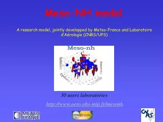
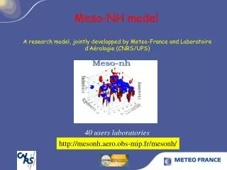
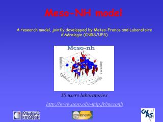
Meso-NH model. A research model, jointly developped by Meteo-France and Laboratoire d’Aérologie (CNRS/UPS). 30 users laboratories. http://www.aero.obs-mip.fr/mesonh. Examples of Applications of Meso-NH. General description of Meso-NH Grid nesting

Meso-NH model
E N D
Presentation Transcript
Meso-NH model A research model, jointly developped by Meteo-France and Laboratoire d’Aérologie (CNRS/UPS) 30 users laboratories http://www.aero.obs-mip.fr/mesonh
Examples of Applications of Meso-NH • General description of Meso-NH • Grid nesting • Clouds representation (explicit convective clouds, Sc) • Cyclones • Coupling with the surface • Coupling with other models (hydrology, dispersion) • Diagnostics • Systematic validations (climatology, real time runs) • Towards AROME
General description of Meso-NH • Anelastic equations with the pseudo-incompressible system of Durran • Vertical coordinate following the terrain : (Gal Chen and Sommerville, 1975) • Temporal discretization : Purely explicit leap-frog scheme • Advection scheme : 2nd order eulerian schemes • Spatial discretization : Arakawa C grid • Grid nesting : One-way/Two-way • Initial fields and LBC (radiative open) from ECMWF/ARPEGE/ALADIN. DYNAMICS • Turbulence : 1.5 order closure Cuxart-Bougeault-Redelsperger (2000) • Convection : Kain-Fritsch (1993) revised by Bechtold et al. (2001) • Microphysical scheme : Bulk schemes at 1-moment or 2-moments. Up to 7 prognostic species: vapor (rv), cloud (rc), rain (rr), pristine ice (ri), snow (rs), graupel (rg), hail (rh) • Radiation : ECMWF package • Chemical on-line scheme : Gazeous and aerosols (Presentation C.Mari, Thursday) • Externalized surface model(Presentation P.Le Moigne, this afternoon) PHYSICS
Types of simulations • A broad range of resolution from synoptic scales (Dx~10km) to meso-scale (Dx~1km) to Large Eddy Simulation (Dx~10m) • Real cases (from ECMWF, ARPEGE, ALADIN analyses or forecasts) • Ideal cases unrealistic cases • - Academic cases (validation of the dynamics) • - Basic studies (Diurnal cycle …) : Cloud Resolving Model (CRM) • - To reproduce an observed reality (via forcings) • (intercomparison : GCSS, EUROCS …) • Simulations 3D, 2D, 1D
Grid nesting technics A single constraint : an integer ratio between the resolutions and the time steps Same vertical grids. At every time step : The Coarse Model (CM) gives the lateral boundary conditions to Fine Model (FM) by interpolation One-way : the FM doesn’t influence the CM Two-way : CM fields are relaxed to the average of FM fields
Vaison-la-Romaine : 22 september 1992 One-way Two-way 3 nested grids : 40/10/2.5km Instantaneous precipitations 2.5km Stein et al., 2000
Vaison-la-Romaine : 22 september 1992 One-way Two-way 2.5 km Cumulated precipitations for 9h (Obs=300mm en 6h) 10km Stein et al., 2000
Examples of Applications of Meso-NH • General description of Meso-NH • Grid nesting • Clouds representation (explicit convective clouds, Sc) • Cyclones • Coupling with the surface • Coupling with other models (hydrology, dispersion) • Diagnostics • Systematic validations (climatology, real time runs) • Towards AROME
Mixed phase cloud representation with a bulk scheme Ice crystals Snowflakes Graupel Hail Cloud droplets Mixed phase : 0°C 0°C Cloud droplets Raindrops Liquid phase : Cloud properties = f( , , , , , )
The different processes Nucleation Autoconversion Deposition Riming Aggregation Freezing 0°C 0°C Collection Collection Melting Sedimentation
Instantaneous precipitation 2.5km 2-way without ICE 2-way with ICE Stein et al., 2000
U Convective Stratiform W H D Density Current q A tropical squall line (P.Jabouille) : Idealized simulation according to a real case (COPT81) Lafore Moncrieff 89
Cloud droplets Rain drops Graupel Pristine ice Snow Jabouille. Caniaux et al., 1994
Three contrasted MAP cases IOP 8 Stratiform rain IOP 3 Moderate Convection IOP 2A Strong Convection F.Lascaux and E.Richard, 2005
Microphysical retrievals : IOP 2A (intense convection) 18:00 UT 12 km 19:00 UT 20:00 UT (x) hail + graupel Z > 60 dBz (o) hail ( ) rain 100 km Tabary, 2002
Hydrometeor type Radar Retrieval (S-Pol) Simulation (Meso-NH) 18:00 UT 12 km 19:00 UT (x) hail + graupel (o) hail 20:00 UT (x) hail + graupel graupel hail (o) hail rain rain 100 km
dry snow hail + graupel rain Pujol et al., 2005 Microphysical retrievals - IOP 3 (moderate convection) 18:10 UT 18:30 UT
Microphysical retrievals - IOP 3 (moderate convection) hail + graupel S-Pol retrieval Meso-NH simulation snow snow rain rain
Microphysical retrievals - IOP 8 (stratiform rain) S-Pol retrieval Meso-NH simulation snow rain melting snow Medina et Houze, 2003
Microphysical budgets : Mean vertical distribution of the hydrometeors ice snow hail cloud rain IOP 2A IOP 3 graupel IOP 8 snow cloud Lascaux et al., 2005 rain
Microphysical budgets : mean vertical distribution of the different processes ice rain IOP 8 IOP 3 IOP 2A
MESO-NH, x=2.5km m MESO-NH, x=2.5km max : 99 mm Initialisation Ducrocq et al (2000)’s max: 31 mm Quasi-stationnary MCS 13-14 Oct. 1995 MESO-NH, x=10km OBSERVATIONS m mm max : 25 mm max : 135 mm Initial conditions: ARPEGE analysis at 18UTC Cumulated precipitation 01 UTC to 06 UTC the 14th Oct. 1995 (Ducrocq et al, 2002)
Gard flash-flood (8-9 Sept.2002) Sensitivity to initial conditions MESO-NH (2.5km) Initial Conditions : Ducrocq et al (2000) Initialisation 12UTC, 08/09/02 Initial Conditions : ARPEGE analysis 12UTC, 08/09/02 + Nîmes + + Ducrocq V, F.Bouttier Météo-France SRNWP/Met Office/Hirlam workshop on Variational Methods Exeter (UK) 15-17 Nov 2004 Raingauges + Nîmes (Ducrocq et al, 2004) Observations Nîmes radar 12-h accumulated précipitation from 12 UTC, 8 Sept to 00 UTC, 9 Sept 2002
The approach Model towards Satellite to validate the cloud coverage TROCCINOX 2005Chaboureau et al., 2005 Cirrus Convection Méso-NH Tb 10.8 m Diff 8.7 - 10.8 m Observation Geophysica
Cloud water mixing ratio (kg/kg) Max = 0.6 g/kg LES simulation of the diurnal cycle (Dx=50m) altitude (m) Min = 0.025 g/kg 0h 12h 0h 12h 0h Observations of the base and the top cloud layer Stratocumulus : Capped BL When the CBL is blocked by an anticyclonic subsidence FIRE 1 case of EUROCS : Forcing terms : a LS subsidence + cooling (dql/dt<0) and moistening (dqt/dt>0) under the inversion to balance the subsidence Sandu et al., 2006
Examples of Applications of Meso-NH • General description of Meso-NH • Grid nesting • Clouds representation (explicit convective clouds, Sc) • Cyclones • Coupling with the surface • Coupling with other models (hydrology, dispersion) • Diagnostics • Systematic validations (climatology, real time runs) • Towards AROME
7800 km, Dx=36km 1944 km , Dx=12km 720km , Dx=4km 3600km Simulation of cyclone : case of Dina Automatic method of Initialization : Filtering/Bogussing Barbary et al.
Simulations CEPMMT : trajectoires 22/01/02 00 UTC Barbary et al.
Évolution en intensité Barbary et al.
Vertical cross-sections at Dx=4km K K m/s m/s W-E S-N Horizontal wind Barbary et al.
Fine scale structure (1 km) le 22 janvier 17h10-17h20-17h30 dBZ Radar reflectivity 10-3s-1 Relative vorticity
Examples of Applications of Meso-NH • General description of Meso-NH • Grid nesting • Clouds representation (explicit convective clouds, Sc) • Cyclones • Coupling with the surface • Coupling with other models (hydrology, dispersion) • Diagnostics • Systematic validations (climatology, real time runs) • Towards AROME
EXTERNALIZED SURFACE : Exchange of data flow at each time step between the 2 models Boundary conditions for turbulence and radiative schemes Méso-NH AROME Arpège / Aladin albedo emissivity radiative temperature fluxes : Momentum, heat, water vapor, CO2, chemistry Atmosphere forcing Sun position Radiative fluxes SURFACE Lake Town Sea Nature Presentation of P.Le Moigne
3D Meso-NH simulations (Lemonsu et al., 2004, 2005) (m) (m) 2000 (m) 2000 2000 1000 1000 France 1000 500 500 Model 1 500 200 200 Marseille 200 100 100 100 50 Model 3 (m) Mer Mediterranée 50 Model 4 50 Mer Mediterranée 700 Mer Mediterranée 600 500 City centre 400 300 Model 2 Marseille 200 Massif du Puget Mediterranean Sea 100 50 Marseille veyre • Set-up : • 4 grid-nesting models from regional to city scale, with respective resolutions of 12 km, 3 km, 1 km and 250 m Chaine de l’Etoile Validation of simulations at urban scale Validation of simulations at regional scale N.D. de la Garde Mont St-Cyr Marseilleveyre Puget
2500 2500 Obs 2000 2000 1500 1500 Altitude (m) Altitude (m) 1000 1000 500 500 Model 25 juin 26 juin 21 juin 22 juin 23 juin 24 juin Regional validation Radiosoundings St Rémy de Provence St Rémy
Thermodynamic structures Air temperature inside the streets 26 June 2001, 1400 UTC Urban network Model Lemonsu et al., 2005a
ZS (m) 3 km Etoile Massif 500 VAL (Lidar) 400 190o 300 OBS (Radar) 200 Puget Massif CNRS (Radar) 100 -6 -4 -2 0 2 4 6 m s-1 Marseilleveyre 50 Comparison with transportable wind lidar (TWL) 26 June 2001, 1400 UTC 2.5 Model TWL D D 2.0 C C 1.5 W Altitude (km) B 1.0 B A 0.5 City center City center A VDOL VDOL 0 2 4 6 0 2 4 6 Distance (km) Distance (km) Lemonsu, Bastin et al., 2005b
Atmospheric boundary layer Horizontal wind field 26 June 2001, 1400 UTC z = 50 m AGL z = 400 m AGL m s-1 VAL VAL West SSB OBS OBS City centre City centre Puget Massif Puget Massif CNRS CNRS South-East DSB South SSB Marseilleveyre Marseilleveyre
Simulation on PARIS DAY Without town Realistic q TKE Dx=1km Lemonsu et Masson (2001)
Nocturnal UBL q Without town Realistic Lemonsu et Masson (2001)
Formation of fog Masson (2001)
Meso-NH Surface Met. forcing LE, H, Rn, W, Ts… ISBA-A-gs Anthropogenic Sea CO2 Flux [CO2]atm CarboEurope/RE : modélisation Meso-NH/ISBA-A-gs C.Sarrat et al., CNRM/GMME/MC2 Modelisation of the atmospheric CO2 in interaction with the surface : coupling of CO2 in Meso-NH with CO2 fluxes of ISBA-A-gs • Improvement of the exchanges surface-atmosphere • Improvement of water cycle/ evapotranspiration • Improvement of the PBL representation • Regional budget of CO2 atmosphérique • Inversion of CO2 concentrations to identify sources/sinks of CO2 (Thèse T. Louvaux)
Modélisation 3-D : Configuration Nesting 2 ways Surface : ISBA-A-gs (Ecoclimap) Vertical grid : 60 levels (0 -14000m) Domaine : Landes (320x250 km) Résolution horizontale : 2.5 km Pas de temps : T = 5 s Domaine : France (900x900 km) Résolution horizontale : 10 km Pas de temps : T = 10 s
Modélisation 3-D : Résultats SFCO2 RN LE [CO2] H
CarboEurope/RE : modelisation Meso-NH/ISBA-A-gs and atmospheric CO2 [CO2] simulated at 15H (june 2001) Advection + Assimilation + vertical mixing [CO2] decrease 00H : Advection + Respiration + cooling [CO2] increase
Coupling of Meso-NH with other models (Hydrology, Dispersion)
Ardèche Cèze Gard Vidourle HYDROLOGY : Development of the coupling Meso-NH-ISBA-TOPMODEL K.Chancibault et al., CNRM/GMME/MICADO • TOPMODEL (Beven and Kirkby, 1979) distributed hydrologic model with one model by basin : 9 basins (200-2200 km²) • Objectives : - Flow and rapide flood forecasts - Retroaction of the hydrology on the atmosphere - Available for AROME
t = 5 min x = 2-3 km L = 1000 km Meso-NH ou Arome Strategy of the coupling flux Wmob ISBA TOPMODEL t = 5 min x = 2-3 km L = 1000 km t = 1h x = 50 m L = 1 km Module de routage
120km, Dx=2km 30km, Dx=500m Dispersion with passive tracers : case of AZF Tulet et Lac (2001)