Interval Estimates in Industrial Engineering: Understanding Estimation
Learn about interval estimates in industrial engineering, estimation techniques, and confidence intervals for unknown variables. Gain insight into sample sizes and precision calculations. Example scenarios included.

Interval Estimates in Industrial Engineering: Understanding Estimation
E N D
Presentation Transcript
s » m X N ( , ) n Interval Estimates • Suppose our light bulbs have some underlying distribution f(x) with finite mean m and variance s2. Regardless of the distribution, recall from that central limit theorem that
a/2 a/2 1 - a za/2 za/2 0 - a = - £ £ 1 P ( z Z z ) a a / 2 / 2 Interval Estimates • Recall that for a standard normal distribution,
- m X = » Z N ( 0 , 1 ) s n s » m X N ( , ) n - m x - a = - £ £ 1 P ( z z ) s a a / 2 / 2 n Interval Estimates But, so, Then,
s s = - £ - m £ P ( z x z ) a a / 2 / 2 n n s s = - - £ - m £ - - P ( x z x z ) - m x a a / 2 / 2 - a = - £ £ n n 1 P ( z z ) s a a / 2 / 2 n Interval Estimates
s s = + ³ m ³ - P ( x z x z ) a a / 2 / 2 n n s s = - - £ - m £ - - P ( x z x z ) a a / 2 / 2 n n Interval Estimates 1 - a
s s = + ³ m ³ - P ( x z x z ) a a / 2 / 2 n n Interval Estimates 1 - a In words, we are (1 - a)% confident that the true mean lies within the interval s ± x z a / 2 n
100 ± 1 , 596 1 . 645 25 ± 1 , 596 32 . 9 Example • Suppose we know that the variance of the bulbs is given by s2 = 10,000. A sample of 25 bulbs yields a sample mean of 1,596. Then a 90% confidence interval is given by
Example or 1,563.1 < m < 1,628.9 32.9 1,563.1 1,596 1,628.9
s = E z a / 2 n Example or 1,563.1 < m < 1,628.9 32.9 1,563.1 1,596 1,628.9 32.9 is called the precision (E) of the interval and is given by
1,596 1,578 1,612 1,584 Example • Suppose we repeat this process 4 times and get 4 sample means of 1596, 1578, 1612, and 1584. Computing confidence intervals then gives
1,596 1,578 1,612 1,584 Interpretation • Either the mean is in the confidence interval or it is not. A 90% confidence interval says that if we construct 100 intervals, we would expect 90 to contain the true mean m and 10 would not.
100 ± 1 , 596 2 . 575 25 ± 1 , 596 51 . 5 A Word on Confidence Int. • Suppose instead of a 90% confidence, we wish to be 99% confident the mean is in the interval. Then
A Word on Confidence Int. • That is, all we have done is increase the interval so that we are more confident that the true mean is in the interval. 32.9 90% Confidence 99% Confidence 1,563.1 1,596 1,628.9 51.5 1,544.5 1,596 1,647.5
Sample Sizes • Suppose we wish to compute a sample size required in order to have a specified precision. In this case, suppose we wish to determine the sample size required in order to estimate the true mean within + 20 hours.
s = E z a / 2 n 2 s æ ö z = a ç ÷ / 2 n E è ø Sample Sizes • Recall the precision is given by Solving for n gives
2 æ ö 1 . 645 ( 100 ) = ç ÷ n 20 è ø = = 67 . 65 68 Sample Sizes • We wish to determine the sample size required in order to estimate the true mean within + 20 hours with 90% confidence.
2 æ ö 1 . 645 ( 100 ) = ç ÷ n 20 è ø = = 67 . 65 68 Sample Sizes • We wish to determine the sample size required in order to estimate the true mean within + 20 hours with 90% confidence. Greater precision requires a larger sample size.
South Dakota School of Mines & TechnologyEstimationIndustrial Engineering
Estimation Interval Estimates(s unknown)Industrial Engineering
n å 2 - 2 x n x i = 2 = i 1 s - n 1 Confidence Intervals s unknown • Suppose we do not know the true variance of the population, but we can estimate it with the sample variance.
n å 2 - 2 x n x i = 2 = i 1 s - n 1 Confidence Intervals (s unknown) • Suppose we do not know the true variance of the population, but we can estimate it with the sample variance. For large samples (>30), replace s2 with s2 and compute confidence interval as before.
- m x = » t t - 1 n s n Confidence Intervals (s unknown) • For small samples we need to replace the standard normal, N(0,1) , with the t-distribution. Specifically,
tn-1 - m a/2 a/2 x = » t t 1 - a - 1 n s n tn-1,a/2 tn-1,a/2 0 Confidence Interval (s unknown)
tn-1 - m a/2 a/2 x = » t t 1 - a - 1 n s n tn-1,a/2 tn-1,a/2 0 Confidence Interval (s unknown) Assumption: x is normally distributed
tn-1 a/2 a/2 1 - a tn-1,a/2 tn-1,a/2 0 - m x - a = - £ £ 1 P ( t t ) - a - a 1 , / 2 1 , / 2 n n s n Confidence Interval (s unknown)
- m x s - a = - £ £ 1 P ( t t ) ± x t - a - a 1 , / 2 1 , / 2 n n s - a 1 , / 2 n n n Confidence Interval (s unknown) Miracle 17b occurs
100 ± 1 , 596 1 . 711 s 25 ± x t - a 1 , / 2 n n Example • Suppose in our light bulb example, we wish to estimate an interval for the mean with 90% confidence. A sample of 25 bulbs yields a sample mean of 1,596 and a sample variance of 10,000.
100 ± 1 , 596 1 . 711 s 25 ± x t - a 1 , / 2 n n Example • Suppose in our light bulb example, we wish to estimate an interval for the mean with 90% confidence. A sample of 25 bulbs yields a sample mean of 1,596 and a sample variance of 10,000. 1,596 + 34.2
32.9 1,563.1 1,596 1,628.9 34.2 1,561.8 1,596 1,630.2 Example • Note that lack of knowledge of s gives a slightly bigger confidence interval (we know less, therefore we feel less confident about the same size interval). s known s unknown
-4.00 -2.00 0.00 2.00 4.00 A Final Word N(0,1) t10
-4.00 -2.00 0.00 2.00 4.00 A Final Word N(0,1) t20
-4.00 -2.00 0.00 2.00 4.00 A Final Word N(0,1) t30
® t z - a a n 1 , / 2 / 2 A Final Word • Note that on the t-distribution chart, as n becomes larger, hence, for larger samples (n > 30) we can replace the t-distribution with the standard normal.