Point and Interval Estimates
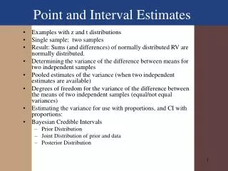
Point and Interval Estimates. Examples with z and t distributions Single sample; two samples Result: Sums (and differences) of normally distributed RV are normally distributed. Determining the variance of the difference between means for two independent samples

Point and Interval Estimates
E N D
Presentation Transcript
Point and Interval Estimates • Examples with z and t distributions • Single sample; two samples • Result: Sums (and differences) of normally distributed RV are normally distributed. • Determining the variance of the difference between means for two independent samples • Pooled estimates of the variance (when two independent estimates are available) • Degrees of freedom for the variance of the difference between the means of two independent samples (equal/not equal variances) • Estimating the variance for use with proportions, and CI with proportions: • Bayesian Credible Intervals • Prior Distribution • Joint Distribution of prior and data • Posterior Distribution
Introduction to Biostatistics (PUBHLTH 540) Examples of Point and Interval Estimates+ Credibility Intervals Examples from Seasons Study • Assumptions: Subjects are SRS from population. • Assume different groups are independent SRS from different stratum (ie. gender) Details: • Use t-distribution for interval estimates when sample sizes are small (unless estimate is of a proportion) • requires an assumption that the underlying random variable is normally distributed • When response is binary (yes/no), we estimate the population mean by the sample mean (equal to the sample proportion ), and the sample variance by
Examples: Point and Interval Estimate of Wt Examples from Seasons Study (see ejs09b540p34.sas). What is a 95% Confidence Interval for Weight? (see: http://dostat.stat.sc.edu/prototype/calculators/index.php3 )?dist=T to get t-percentiles) Use applets to get t value The mean weight is estimated as 77.6 kg, with a 95% CI of (75.6, 79.7)
Examples: Point and Interval Estimate of Wt • Suppose we assume the Seasons study subjects were a SRS from people in the US. What is a point and interval estimate of weight for the US population? Answer: Same as before--The mean weight is estimated as 77.6 kg, with a 95% CI of (75.6, 79.7)
Examples: Point and Interval Estimate of Wt- separately for men and women Table 3. Description of weight by gender Male(0) Analysis Variable : wt Wt (kg) (formerly cc5a) N Mean Std Dev Variance Std Error ƒƒƒƒƒƒƒƒƒƒƒƒƒƒƒƒƒƒƒƒƒƒƒƒƒƒƒƒƒƒƒƒƒƒƒƒƒƒƒƒƒƒƒƒƒƒƒƒƒƒƒƒƒƒƒƒƒƒƒƒƒƒƒƒƒƒƒ 142 85.90 15.82 250.32 1.33 ƒƒƒƒƒƒƒƒƒƒƒƒƒƒƒƒƒƒƒƒƒƒƒƒƒƒƒƒƒƒƒƒƒƒƒƒƒƒƒƒƒƒƒƒƒƒƒƒƒƒƒƒƒƒƒƒƒƒƒƒƒƒƒƒƒƒƒ Female(1) Analysis Variable : wt Wt (kg) (formerly cc5a) N Mean Std Dev Variance Std Error ƒƒƒƒƒƒƒƒƒƒƒƒƒƒƒƒƒƒƒƒƒƒƒƒƒƒƒƒƒƒƒƒƒƒƒƒƒƒƒƒƒƒƒƒƒƒƒƒƒƒƒƒƒƒƒƒƒƒƒƒƒƒƒƒƒƒƒ 149 69.73 15.92 253.42 1.30 ƒƒƒƒƒƒƒƒƒƒƒƒƒƒƒƒƒƒƒƒƒƒƒƒƒƒƒƒƒƒƒƒƒƒƒƒƒƒƒƒƒƒƒƒƒƒƒƒƒƒƒƒƒƒƒƒƒƒƒƒƒƒƒƒƒƒƒ Source: ejs09b540p34.sas 10/20/2009 by ejs Examples from Seasons Study ejs09b540p34.sas (see: http://dostat.stat.sc.edu/prototype/calculators/index.php3?dist=T to get t-percentiles) Use Applet-- men Use Applet-- women For men, the mean weight is estimated as 85.9 kg (95% CI (83.3,88.5) while for women, mean wt is 69.7 kg (95% CI (67.2, 72.3)
Examples: Point and Interval Estimate of Wt- adjusting for gender in US population • Suppose we assume the Seasons study male subjects were a SRS from males in the US, and similarly, and female subjects were an independent SRS from females in the US. In 2000, there were 138.05 million males, and 143.37 million females in the U.S.. Using the Seasons study estimates, what is a point and interval estimate of weight for the US population? Males Females
Example: Linear Combinations of Random variables What are the DF for the t-dist? If variances are equal, use df=n1+n2-2, and replace individual variance estimates by a pooled variance. If variances are not equal, see p270-271 in text for df approximation.
Note: Common estimate of a variance- Pooled Estimate If we assume the population variance in weight is equal for males and females, we can estimate a pooled (common) variance (see p267 in text): More generally: for Wt:
Example: Linear Combinations of Random variables Assuming not equal: from p270-271 in text,
Example: Linear Combinations of Random variables Wt is estimated as 77.6 kg with a 95% CI of (75.8,79.5)
Examples: Proportion of Subjects who are obese (BMI>30) (see p327 text) • Estimate the proportion of subjects obese, and a 95% CI • Create 0/1 variable 1=obese 0=normal wt • Use Z-dist for CI (since np>5) • Variance estimate: See: ejs09b540p34.sas
Examples: Proportion of Subjects who are obese (BMI>30) (see p327 text) • Single random variable (0/1) is called a Bernoulli random variable. • Variance is estimated using maximum likelihood estimator (biased): • Usual estimate of the variance (used in other settings) is: • Normal Approximation is used commonly when nP>5 and n(1-P)>5 (NOT t-dist) Example: Sample finds 4 of 10 subjects obese 95% CI Note: nP is not large enough here for the normal approximation to be “good”.
Examples: Credible IntervalsBayesian Approach Recall that we could estimate the mean using Maximum Likelihood Example: We select a srs with replacement of n=10 and observe x=4. What is p? Solution 1: Use the sample mean: Solution 2: Use value of the parameter p that maximizes the likelihood, given the data. Likelihood: The likelihood is a function of p. We can think of a set of possible values, i.e. 0, 0.1, 0.2, …, 0.8, 0.9, 1 of p. The maximum likelihood estimate is the value of p where the likelihood is largest.
We select a srs with replacement of n=10 and observe x=4. What is p? Binomial DistributionLikelihood
Likelihood: Binomial DistributionMaximum Likelihood Maximum Likelihood 0.2 0.1 0.05 0.2 0.3 0.4 0.5 0.6 0.7 0.9
Examples: Credible IntervalsBayesian Approach-Prior Suppose we assume each parameter is equally likely. This is called a uniform prior distribution Prior distribution
We select a srs with replacement of n=10 and observe x=4. The likelihood is the Pr(Data|p) Examples: Credible IntervalsBayesian Approach-Data|p
Combining the Likelihood and the prior, we have the joint probabilities Examples: Credible IntervalsBayesian Approach-Posterior We sum these probabilities over all possible possible values of p, and divide by this sum to form posterior probabilities:
Examples: Credible IntervalsBayesian Approach-Posterior Credible Intervals are like Confidence Intervals for parameters in the Posterior Distribution (Uniform Prior)
Examples: Credible IntervalsBayesian Approach-Posterior Credible Intervals are like Confidence Intervals for parameters in the Posterior Distribution (Symmetric Prior)
Examples: Credible IntervalsBayesian Approach-Posterior Credible Intervals are like Confidence Intervals for parameters in the Posterior Distribution (Tiered Prior)
Examples: Credible IntervalsBayesian Approach-Conclusions Credible Intervals (for the same data) depend on the Prior Distribution Prior Credible Interval Confidence Uniform (0.15, 0.70) 0.96 Symmetric (0.15, 0.35) 0.91 Tiered (0.15, 0.55) 0.89 Frequentist 95% Confidence Intervals based on Normal Approximation (0.10, 0.70) Credible Interval- Intuitive Interpretation- prob parameter is in interval is confidence Frequentist Confidence Interval- awkward interpretation- includes parameter for 95% of samples, if repeated