Understanding Interval Estimates and Hypothesis Testing in OLS: Assessing Coefficient Reliability
150 likes | 265 Vues
This lecture explores the concepts of interval estimates and hypothesis testing, focusing on the reliability of coefficient estimates in ordinary least squares (OLS) regression. It discusses the differences between the normal and Student's t-distributions, outlining how to assess the reliability of estimates, evaluate coefficient variance, and determine confidence in the relationship between study time and quiz scores. By employing these statistical methods, students will learn to formalize hypothesis testing and gain insights into more accurate modeling of educational performance.

Understanding Interval Estimates and Hypothesis Testing in OLS: Assessing Coefficient Reliability
E N D
Presentation Transcript
Lecture 2.4 Preview: Interval Estimates and Hypothesis Testing Clint’s Assignment: Taking Stock Estimate Reliability: Interval Estimate Question Normal Distribution versus the Student t-Distribution: One Last Complication Assessing the Reliability of a Coefficient Estimate: Applying the Student t-Distribution Theory Assessment: Hypothesis Testing Motivating Hypothesis Testing: The Cynic Formalizing Hypothesis Testing: The Steps Summary: The Ordinary Least Squares (OLS) Estimation Procedure Standard Ordinary Least Squares (OLS) Premises Ordinary Least Squares (OLS) Estimation Procedure: Three Important Parts Properties of the Ordinary Least Squares Estimation Procedure
Clint’s Assignment: Taking Stock Theory: Studying more results in higher quiz scores. The Model:yt = Const + xxt+ et yt = Actual quiz score xt = Minutes studied et = Error term Const = Points given for showing up x = Points earned for each minute studied Clint wishes to find the values of Const and x? But Const and x are not observable. Clint can never determine the actual values of Const and x. How can he proceed? First Quiz Student x y 1 5 66 2 15 87 3 25 90 Ordinary Least Squares (OLS) Estimates Esty = 63 + 1.2x bConst = 63 = Estimated points given for showing up bx = 1.2 = Estimated points for each minute studied Clint’s Assignment Coefficient Reliability: How reliable is the coefficient estimate, 1.2, calculated from the first quiz? That is, how confident should Clint be that the coefficient estimate, 1.2, will be close to the actual value? Theory Confidence: How much confidence should Clint have in the theory that additional studying increases quiz scores?
General Properties of the Ordinary Least Squares (OLS) Estimation Procedure When the standard ordinary least squares premises are met, the following equations describe the coefficient estimate’s probability distribution: Mean[bx] = x Var[bx] = Importance of the Probability Distribution’s Mean (Center) and Variance (Spread) Mean: When the mean of the coefficient estimate’s probability distribution, Mean[bx], equals the actual value of the coefficient, x, the estimation procedure is unbiased. Unbiased does not mean that the estimate will equal the actual value. In fact, we can be all but certain that the estimate will not equal the actual value. Unbiased does mean that the estimation procedure does not systematically underestimate or overestimate the actual coefficient value. Formally, the mean of the estimate’s probability distribution equals the actual value. For more intuition, suppose that the estimate’s probability distribution is symmetric: the chances that the estimate is too high equals the chances that it is too low. Variance: When the estimation procedure for the coefficient value is unbiased, the variance of the estimate’s probability distribution, Var[bx], determines the reliability of the estimate. As the variance decreases, the estimate is more likely to be close to the actual coefficient value. The Problem: But there is a problem here, isn’t there? Econometrician’s Philosophy: If you lack the information to determine the value directly, estimate the value to the best of your ability using the information you do have.
OLS Estimation Procedure: Three Estimation Procedures The ordinary least squares (OLS) estimation procedure actually includes three procedures: A Procedure to Estimate the Value of the Parameters A Procedure to Estimate the Variance of the Error Term’s Probability Distribution A Procedure to Estimate the Variance of the Coefficient Estimate’s Probability Distribution Good News: When the standard ordinary least squares (OLS) premises are satisfied: Each of the three procedures is unbiased. The procedure to estimate the value of the parameters is the best linear unbiased estimation procedure.
Coefficient Reliability: How reliable is the coefficient estimate, 1.2, calculated from the first quiz? That is, how confident should Clint be that the coefficient estimate, 1.2, will be close to the actual value? Interval Estimate Question: What is the probability that the coefficient estimate, 1.2, lies within _____ of the actual coefficient value? _____. One Last Complication We do not know the actual value of the variance for the coefficient estimate’s probability distribution. To use the normal distribution we must know the actual value of the variance (and the standard deviation) for the random variable’s probability distribution. We must estimate its variance. We cannot use the normal distribution when dealing with the coefficient estimate. Instead we must use another distribution, the Student t-distribution.
The Normal Distribution Versus the Student t-Distribution Student t-distribution: t equals the number of estimated standard deviations the value lies from the mean. Normal distribution: z equals the number of standard deviations the value lies from the mean. Student t-distribution Normal distribution Standard deviation is not known Standard deviation is known Standard deviation must be estimated PRS 1-3 Mean Since we must estimate the value of the standard deviation, we are introducing an additional element of uncertainty into the mix. Why is the Student t-distribution more “spread out?” Hence, the Student t-distribution more “spread out” than the normal distribution. Furthermore, the Student t-distribution is more complicated than the normal distribution: its “spread” depends on the degrees of freedom.
The Normal Distribution’s z and the Student t-Distribution’s t When the standard deviation is known, use the normal distribution: Value of Random Variable Mean of Random Variable z = Standard Deviation of Random Variable = Number of Standard Deviations from the Mean When the standard deviation must be estimated, use the t-distribution: Value of Random Variable Mean of Random Variable t = Estimated Standard Deviation of Random Variable = Number of Estimated Standard Deviations (Standard Errors) from the Mean t-distribution is affected by the degrees of freedom. Coefficient Reliability: How reliable is the coefficient estimate, 1.2, calculated from the first quiz? That is, how confident should Clint be that the coefficient estimate, 1.2, will be close to the actual value? Interval Estimate Question: What is the probability that the coefficient estimate, 1.20, lies within _____ of the actual coefficient value? _____. 1.50 First Blank: We begin by filling in the first blank, choosing our “close to” value. Suppose that we choose 1.50; Close To Criterion = 1.50 So we write 1.50 in the first blank.
Interval Estimate Question: What is the probability that the coefficient estimate, 1.20, lies within _____ of the actual coefficient value? _____. 1.50 .78 Convert 1.50 into standard errors: Second Blank: Calculate the probability. Probability that the estimate lies within 1.50 of the actual value 1.50 Question: Why does the actual value equal the distribution mean? = 2.89 .5196 .78 t = Number of standard errors from the mean Answer: The ordinary least squares (OLS) estimation procedure is unbiased. .11 .11 Left tail: LabLink 1.50 1.50 Right tail: LabLink 2.89 SE’s 2.89 SE’s x 1.50 x + 1.50 Actual Value = x t = 2.89 t = 2.89 Degrees Number of = Sample Size of EstimatedFreedom Parameters = 3 2 = 1 Probability that the estimate lies within 1.50 of the actual value equals Probability that the estimate lies within 2.89 SE’s of the actual value Between t‘s of 2.89 and +2.89 = 1.00 .22 = .78 = 1.00 (.11 + .11)
Clint’s Assignment: Theory Confidence. How much confidence should Clint have in the theory that additional studying increases quiz scores? Theory: Additional studying increases quiz scores. Step 0: Construct a model reflecting the theory to be tested yt = Const + xxt + et yt = Actual quiz score xt = Minutes studied et = Error term Const reflects points given for showing up x reflects points earned for each minute studied First Quiz Student xy 1 5 66 2 15 87 3 25 90 The theory suggests that x should be positive. Step 1: Collect data, run the regression, and interpret the estimates bConst = Estimate of Const = 63 The estimated equation: Esty = 63 + 1.2x bx = Estimate of x = 1.2 Interpretation: The regression suggests that students receive 63 points for showing up 1.2 additional points for each minute studied Critical Result: The parameter estimate evidence suggests that the theory postulating the benefits of additional studying is correct. The coefficient estimate is positive. More specifically, the coefficient estimate lies 1.2 above 0.
Step 2: Play the cynic and challenge the results; construct the null and alternative hypotheses: Cynic’s view: Sure, the coefficient estimate was positive, but this result was just “the luck of the draw.” In fact, studying has no impact on quiz scores, the actual coefficient, x, equals 0. H0: x = 0 Cynic is correct: Studying has no impact on a student’s quiz score H1: x > 0 Cynic is incorrect: Additional studying increases quiz scores PRS 4 Question: Can we dismiss the cynic’s view as being impossible? No LabLink 8.1 Step 3: Formulate the question to assess the cynic’s view, to assess the null hypothesis. Generic Question: What is the probability that the results would be like those we actually obtained (or even stronger), if the cynic is correct and studying actually has no impact? Specific Question: The regression’s coefficient estimate was 1.2. What is the probability that the coefficient estimate, bx, in one regression would be 1.2 or more, if H0 were true (if the actual coefficient, x, equaled 0)? PRS 5 Answer: Prob[Results IF Cynic Correct] or equivalently Prob[Results IF H0 True] Prob[Results IF H0 True] small Prob[Results IF H0 True] large Unlikely that H0 is true Likely that H0 is true Reject H0 Do not reject H0
H0: x = 0 Cynic is correct: Studying has no impact on quiz score H1: x > 0 Cynic is incorrect: As studying increases, the quiz score increases Step 4: Use the estimation procedure’s general properties to calculate Prob[Results IF H0 True]. Estimate was 1.2: What is the probability that the coefficient estimate in one regression would be 1.2 or more, if H0 were true (if the actual coefficient, x, equaled 0)? OLS estimation procedure unbiased If H0 were true Standarderror Number of observations Number of parameters Mean[bx] = x = 0 SE[bx] = .5196 DF = 3 2 = 1 Question: What do we know about the probability distribution of the coefficient estimates, bx? t-distribution Mean = 0 SE = .5196 DF = 1 Use the Econometrics Lab. LabLink 8.2 .13 Prob[Results IF H0 True] .13 bx 0 1.2
Using Eviews to Calculate Prob[Results IF H0 True] ] OLS estimator is unbiased Assume cynic is correct EViews SE column Number of observations Number of parameters Mean[bx] = x = 0 SE[bx] = .5196 DF = 3 2 = 1 t-Statistic Column: How many standard errors (number of estimated standard deviations) does the coefficient estimate, 1.2, lie from 0? The estimate, 1.2, lies about 2.3 standard errors from 0. = = 2.309 = t-Statistic Column Tails Probability: What is the “tails probability,” the probability that the coefficient estimate, bx, resulting from one regression would will lie at least 1.2 from 0, if the actual coefficient, x, equaled 0? t-distribution Mean = 0 SE = .5196 DF = 1 .13 .13 Tails Probability .26 bx NB: The Prob. Column is based on the premise that the actual coefficient, x, equals 0. 1.2 1.2 0 1.2 Tails Probability: EViews Prob. Column
t-distribution Mean = 0 SE = .5196 DF = 1 .2601/2 .2601/2 bx 1.2 1.2 0 1.2 Question to Assess Cynic’s View: What is the probability of obtaining a result like the one calculated from the first quiz data (a coefficient estimate, bx, of 1.2 or more), if studying actually has no impact on quiz scores (if the actual coefficient, x, were 0)? t-distribution Mean = 0 SE = .5196 DF = 1 .2601/2 Prob[Results IF H0 True] .13 bx 0 1.2 Tails Probability = .2601
H0: x = 0 Cynic is correct: Studying has no impact on a student’s quiz score H1: x > 0 Cynic is incorrect: As studying increases, quiz score increases Prob[Results IF H0 True] .13 Step 5: Decide on the standard of proof, a significance level The significance level is the dividing line between the probability being small and the probability being large. Prob[Results IF H0 True]Less Than Significance Level Prob[Results IF H0 True]Greater Than Significance Level Prob[Results IF H0 True] small Prob[Results IF H0 True] large Unlikely that H0 is true Likely that H0 is true Reject H0 Do not reject H0 Would we reject H0 at a 1 percent (.01) significance level? No. Would we reject H0 at a 5 percent (.05) significance level? No. Would we reject H0 at a 10 percent (.10) significance level? No. At the “traditional” significance levels, we could not reject the null hypothesis; we cannot reject the notion that studying has no impact on quiz scores.
Summary: Standard Regression Assumptions and the Ordinary Least Squares (OLS) Estimation Procedure The Model:yt = Const + xxt + et Const and x are the parameters yt = Dependent variable xt = Explanatory variable et = Error term Role of the Error Term The error term is a random variable representing random influences: Mean[et] = 0 Standard Ordinary Least Squares (OLS) Premises Error Term Equal Variance Premise: The variance of the error term’s probability distribution for each observation is the same. Error Term/Error Term Independence Premise: The error terms are independent. Explanatory Variable Constant Premise: The explanatory variables, the xt’s, are constants; the explanatory variables, the xt’s, are not random variables. Explanatory Variable/Error Term Independence Premise: The explanatory variables, the xt’s, and the error terms, the et’s, are not correlated. OLS Estimation Procedure Includes Three Estimation Procedures Good News: When the standard OLS regression assumptions are met each of these procedures is unbiased. Good News: When the standard OLS regression assumptions are met the OLS estimation procedure is BLUE. Value of the parameters,Const and x: bx = bConst = SSR Variance of the error term’s probability distribution,Var[e]: EstVar[e] = Degrees of Freedom Variance of the coefficient estimate’s probability distribution,Var[bx]: EstVar[bx] =