Download
1 / 29
290 likes | 311 Vues
Learn about point estimates, confidence intervals, sample sizes, and more in statistical inference. Understand how to calculate and interpret confidence intervals for population parameters.

E N D
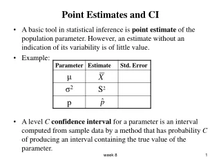
Point Estimates and CI • A basic tool in statistical inference is point estimate of the population parameter. However, an estimate without an indication of its variability is of little value. • Example: • A level Cconfidence interval for a parameter is an interval computed from sample data by a method that has probability C of producing an interval containing the true value of the parameter. week 8
Confidence interval for the population mean • Choose a SRS of size n from a population having unknown mean and known stdev. . A (1- α)100% confidence interval for is an interval of the form, • Here is the value on the standard normal curve with area α to its right. • The interval is exact when the population distribution is normal and approximately correct for large n in other cases. • In general CIs have the form: Estimate margin of error • In the above case, Margin of error = m = week 8
Note, in the above formula for the CI for the population mean, is the stdev. of the sample mean (this is also known as the std. error of the sample mean ). The CI can also be written as • The width of any CI is L = 2m i.e. twice the margin of error. • Here are three ways to reduce the margin of error (and the width of the CI) • Use a lower level of confidence (bigger α). • Increase the sample size n. • Reduce (usually not possible). week 8
Sample size for desired margin of error • The CI for population mean will have a specified margin of error m when the sample size is • Example: A limnologist wishes to estimate the mean phosphate content per unit volume of lake water. It is known from previous studies that the stdev. has a fairly stable value of 4mg. How many water samples must the limnologist analyze to be 90% certain that the error of estimation does not exceed 0.8 mg? Answer: week 8
Exercise • You want to rent an unfurnished one-bedroom apartment for next semester. The mean monthly rent for a random sample of 10 apartments advertised in the local newspaper is $580. Assume that the stdev. is $90. Find a 95% CI for the mean monthly rent for unfurnished one-bedroom apartments available for rent in this community. • How large a sample of one-bedroom apartments would be needed to estimate the mean µ within ±$20 with 90% confidence? week 8
Example • The data below is data on the Degree of Reading Power (DRP) scores for 44 students. 95% CI for the population mean score is given in the MINITAB output below. DRP Scores 40 26 39 14 42 18 25 43 46 27 19 47 19 26 35 34 15 44 40 38 31 46 52 25 35 35 33 29 34 41 49 28 52 47 35 48 22 33 41 51 27 14 54 45 Z Confidence Intervals The assumed sigma = 11.0 Variable N Mean StDev SE Mean 95.0 % CI DRP Scor 44 35.09 11.19 1.66 (31.84 , 38.34) • MINITAB Command Stat > Basic Statistics >1 Sample Z and select ‘Confidence interval’ week 8
Exercise A random sample of 85 students in Chicago city high schools taking a course designed to improve SAT scores. Based on these students a 90% CI for the mean improvement in SAT scores for all Chicago high school students is computed as (72.3, 91.4) points. Which of the following statements are true? • 90% of the students in the sample improved their scores by between 72.3 and 91.4 points. • 90% of the students in the population improved their scores by between 72.3 and 91.4 points. • 95% CI will contain the value 72.3. • The margin of error of the 90% CI above is 9.55. • 90% CI based on a sample of 340 ( 85 X 4) students will have margin of error 9.55/4. week 8
CIs for the population proportion p • Choose an SRS of size n from a population having unknown proportion p of successes. An approximate (1- α)100% confidence interval for p is Again zα is the value on the standard normal curve with area α to its right. • Note 1: Std. error of the sample proportion is = • Note 2: Margin of error of this CI m = • The above CI can be written as • Use this interval when the number of successes and number of failure are both at least 15. week 8
When the sample size is small use either tables of exact CIs or approximate CIs based on Wilson’s estimate given by where, and = • Note, Wilson’s estimate is also called the plus four estimate. • Read Pages 345-347 in textbook. week 8
Example • In a sample of 400 computer memory chips made at Digital Devices, Inc., 40 were found to be defective. Give a 95% confidence interval for the proportion of defective chips in the population from which the sample was taken? week 8
Sample size for desired Margin of error • The level C Confidence interval will have margin of error approximately equal to the specified margin of error m when the sample size n is • Here zα isthe critical value for the confidence level (1- α) and p* is a guessed value for the proportion of successes in a future sample. • The margin of error will be less then or equal to m if p* is chosen to be 0.5. The sample size required is then given by week 8
Example The Gallup Poll asked a sample of 1785 U.S. adults, “Did you, yourself, happen to attend church or synagogue or mosque in the last 7 days?” Of the respondents, 750 said “Yes.” Suppose (it is not, in fact, true) that Gallup's sample was an SRS. (a) Give a 99% confidence interval for the proportion of all U.S. adults who attended church or synagogue or mosque during the week preceding the poll. (b) Do the results provide good evidence that less than half of the population attended church or synagogue or mosque? (c) How large a sample would be required to obtain a margin of error of 0.01 in a 99% confidence interval for the proportion who attend church or synagogue or mosque? (Use Gallup's result as the guessed value of p). week 8
Solution week 8
Exercise Assume that a U.S. study and a Canadian study to estimate the proportion of adults in favor of capital punishment are conducted using simple random samples (not really practical). Assume the true unknown proportions in the 2 countries are fairly similar. The U.S. survey uses a sample 9 times bigger than the Canadian sample. Both samples are quite large. The U.S. population is 9 times bigger than the Canadian population. The Canadian confidence interval will be: a) 9 times wider than the U.S. confidence interval b) 3 times wider than the U.S. confidence interval c) the same width as the U.S. confidence interval d) 9 times smaller than the U.S. confidence interval e) 3 times smaller than the U.S. confidence interval week 8
Statistical tests for the population mean ( known) • A significance test is a formal procedure for comparing observed data with a hypothesis whose truth we want to assess. The hypothesis is a statement about the parameters in a population or model. • Null hypothesis The statement being tested in a test of significance is called the null hypothesis. The test of significance is designed to assess the strength of the evidence against the null hypothesis. Usually the null hypothesis is a statement of “no effect” or “no difference”. • We abbreviate “null hypothesis” as H0 . week 8
Example Each of the following situations requires a significance test about a population mean . State the appropriate null hypothesis H0 and alternative hypothesis Ha in each case. • The mean area of the several thousand apartments in a new development is advertised to be 1250 square feet. A tenant group thinks that the apartments are smaller than advertised. They hire an engineer to measure a sample of apartments to test their suspicion. Answer: (b) Larry's car consume on average 32 miles per gallon on the highway. He now switches to a new motor oil that is advertised as increasing gas mileage. After driving 3000 highway miles with the new oil, he wants to determine if his gas mileage actually has increased. Answer: (c) The diameter of a spindle in a small motor is supposed to be 5 millimeters. If the spindle is either too small or too large, the motor will not perform properly. The manufacturer measures the diameter in a sample of motors to determine whether the mean diameter has moved away from the target. Answer: week 8
Test Statistic • The test is based on a statistic that estimate the parameter that appears in the hypotheses. Usually this is the same estimate we would use in a confidence interval for the parameter. When H0 is true, we expect the estimate to take a value near the parameter value specified in H0. • Values of the estimate far from the parameter value specified by H0give evidence against H0. The alternative hypothesis determines which directions count against H0. • A test statistic measures compatibility between the null hypothesis and the data. • We use it for the probability calculation that we need for our test of significance • It is a random variable with a distribution that we know. week 8
Example • An air freight company wishes to test whether or not the mean weight of parcels shipped on a particular root exceeds 10 pounds. A random sample of 49 shipping orders was examined and found to have average weight of 11 pounds. Assume that the stdev. of the weights () is 2.8 pounds. • The null and alternative hypotheses in this problem are: H0: μ = 10 ; Ha: μ > 10 . • The test statistic for this problem is the standardized version of • Decision: ? week 8
P-value and Significance level • The probability computed under the assumption that H0 is true, that the test statistic would take a value as extreme or more extreme than that actually observed is called the P-value of the test. The smaller the P-value the stronger the evidence against H0 provided by the data. • The decisive value of the P-value is called the significance level. It is denoted by . • Statistical significance If the P-value is as small or smaller than , we reject H0 and say that the data are statistically significant at level . • The P-value is the smallest level α at which the data are significant. week 8
Z Test for a population mean ( known) • To test the hypothesis H0: µ = µ0 based on a SRS of size n from a population with unknown mean µ and known stdev σ, compute the test statistic • In terms of a standard Normal variable Z, the P-value for the test of H0 against Ha : µ > µ0 is P( Z ≥ z ) Ha : µ < µ0 is P( Z ≤ z ) Ha : µ ≠ µ0 is 2·P( Z ≥ |z|) • These P-values are exact if the population distribution is normal and are approximately correct for large n in other cases. week 8
Critical value approach • We can base our test conclusions on a fixed level of significant α without computing the P-value. • For this we need to find a critical value z* from the standard normal distribution with a specified tail area (to the right or left depending on Ha). This tail area is called the rejection region. • If the test statistic falls in the rejection region we reject H0 and conclude that the data are statistically significant at level . • A P-value is more informative then a reject-or-not finding at a fixed significance level because it can tell us about the strength of evidence we found against the H0. week 8
Example • The Pfft Light Bulb Company claims that the mean life of its 2 watt bulbs is 1300 hours. Suspecting that the claim is too high, Nalph Rader gathered a random sample of 64 bulbs and tested each. He found the average life to be 1295 hours. Test the company's claim using = 0.01. Assume = 20 hours. Answer: week 8
Exercise • A standard intelligence examination has been given for several years with an average score of 80 and a standard deviation of 7. If 25 students taught with special emphasis on reading skill, obtain a mean grade of 83 on the examination, is there reason to believe that the special emphasis changes the result on the test? Use = 0.05. week 8
Example • We have data on the Degree of Reading Power (DRP) scores for 44 students. The MINITAB output for the test is given below. Z-Test Test of mu = 32.00 vs mu > 32.00 The assumed sigma = 11.0 Variable N Mean StDev SE Mean Z P DRP Scor 44 35.09 11.19 1.66 1.86 0.031 • MINITAB Command Stat > Basic Statistics >1 Sample Z and select ‘Test mean’ week 8
Confidence Intervals and two-sided tests • A level two-sided significance test rejects a hypothesis H0: μ = μ0 exactly when the value μ0 falls outside the 1- α confidence interval for . • Example For the exercise above (slide 24) a 95% CI is 83 ± 1.96·(7/5) = (80.256, 85.744) The value 80 is not in this interval and so we reject H0: = 80 at the 5% level of significance. week 8
Large sample signif. tests for a population proportion • Draw a SRS of size n from a large population with unknown proportion p of successes. To test the null hypothesis H0: p = p0, compute the z statistic • In terms of a standard normal random variable Z, the approximate p-value for the test of H0 against Ha : p > p0is P( Z ≥ z ) Ha : p < p0is P( Z ≤ z ) Ha : p ≠ p0is 2·P( Z ≥ |z|) • Use the large-sample z test as long as the expected number of successes, np0, and the expected number of failure, n(1- p0), are both greater then 10. week 8
Example Leroy, a starting player for a major college basketball team, made only 38.4% of his free throws last season. During the summer he worked on developing a softer shot in the hope of improving his free-throw accuracy. In the first eight games of this season Leroy made 25 free throws in 40 attempts. Let p be his probability of making each free throw he shoots this season. • State the null hypothesis H0 that Leroy's free-throw probability has remained the same as last year and the alternative Ha that his work in the summer resulted in a higher probability of success. (b) Calculate the z statistic for testing H0 versus Ha. (c) Do you accept or reject H0 for = 0.05 ? Find the P-value. (d) Give a 90% confidence interval for Leroy's free-throw success probability for the new season. Are you convinced that he is now a better free-throw shooter than last season? (e) What assumptions are needed for the validity of the test and confidence interval calculations that you performed? week 8
Solution week 8
MINITAB gives the exact p-value for the test. • Commands: Stats > Basic Statistics > 1 Proportion • MINITAB output for the above example is given below. Test and Confidence Interval for One Proportion Test of p = 0.384 vs p > 0.384 Exact Sample X N Sample p 90.0 % CI P-Value 1 25 40 0.625000 (0.482752, 0.752705) 0.002 week 8