Download
1 / 55
590 likes | 878 Vues
FIGURE 4-1 Some fate and transport processes in the subsurface and atmospheric environment. FIGURE 4-2 Some fate and transport processes in the aquatic environment. FIGURE 4-3 Contaminant transfer through soil-water-air interfaces. FIGURE 4-4

E N D
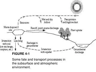
FIGURE 4-1 Some fate and transport processes in the subsurface and atmospheric environment.
FIGURE 4-2 Some fate and transport processes in the aquatic environment.
FIGURE 4-3 Contaminant transfer through soil-water-air interfaces.
FIGURE 4-4 Sources of fluids for the generation of landfill leachate.
FIGURE 4-5 Water balance variables in the HELP model.
FIGURE 4-6 Hydrologic cycle.
FIGURE 4-7 Darcy’s experiment.
FIGURE 4-8 Schematic of saturated flow in laboratory experiment.
FIGURE 4-9 Bernoulli’s equation for flow through a pipe.
FIGURE 4-10 Hydraulic heads in Darcy’s experiment.
FIGURE 4-11 Darcy’s experiment revisited.
FIGURE 4-12 Flow lines and equipotentials.
FIGURE 4-13 Flow net for steady-state flow through a homogeneous embankment.
FIGURE 4-14 Characteristic curves relating hydraulic conductivity and moisture content to pressure head for a naturally occurring sand soil.
FIGURE 4-15 Schematic of mechanical dispersion.
FIGURE 4-16 Effect of dispersion on contaminant transport.
FIGURE 4-17 Plume migration affected by dispersion and source type. The arker the area, the higher the contaminant concentration.
FIGURE 4-18 Effect of diffusion on contaminant transport with no advective transport.
FIGURE 4-19 Schematic of fractured flow.
FIGURE 4-20 Effect of high-permeability zone on contaminant transport.
FIGURE 4-21 Movement of NAPL.
FIGURE 4-22 Two-dimensional control volume.
FIGURE 4-23 Finite difference.
FIGURE 4-24 Simplified flow diagram representing general process of developing a transport model.
FIGURE 4-25 Soil aggregates in subsurface domain.
FIGURE 4-26 Partitioning of sorbate between solvent and sorbent.
FIGURE 4-27 Two-stage sorption model.
FIGURE 4-28 Desorption of sorbate.
FIGURE 4-29 Sorption of lindane by unstripped and stripped soil.
FIGURE 4-30 Variable sorption of trichloroethene on glacial till.
FIGURE 4-31 Solubilities of metal hydroxides as a function of pH.
FIGURE 4-32 Biological transformation of PCE under anaerobic conditions.
FIGURE 4-33 Hydrolysis of chlorinated alkyl compounds.
FIGURE 4-34 Reduction of sorption by cosolvation.
FIGURE 4-35 Effect of the distribution coefficient on contaminant retardation during transport in a shallow groundwater flow system.
FIGURE 4-36 A simplified, expanding box model.
FIGURE 4-37 The effect of turbulent eddies on plumes (after Pendergast, 1984).124 (a) A large cloud in a uniform field of small eddies, (b) a small cloud in a uniform field of large eddies, (c) a cloud in a field of eddies of the same size as the cloud.
FIGURE 4-38 Stable and unstable lapse rates.
FIGURE 4-39 A gaussian distribution.
FIGURE 4-40 Bivariate plume and plume cross section.
FIGURE 4-41 PGT horizontal (crosswind) dispersion coefficient as a function of stability category and downwind distance.
FIGURE 4-42 PGT vertical dispersion coefficient as a function of stability category and downwind distance.
FIGURE 4-43 Two steps of estimating dispersion.
FIGURE 4-44 Relative ground level concentration versus distance.
FIGURE 4-45 Relative ground level concentration versus distance for various stability classes.
FIGURE 4-46 Relative ground level concentration versus distance for various effective stack heights.
EXAMPLE 4-8. FINITE DIFFERENCE SOLUTION FOR DARCY’S EXPERIMENT.
Hydrolysis of chlo-rinated organics involves exchange of the hydroxyl group with an anionic X on a carbon atom.
4-3. The groundwater contours are spaced at intervals of about 50 m.