Download
1 / 103
1.04k likes | 1.08k Vues
Explore atmospheric mercury transport, deposition, & impacts using NOAA HYSPLIT model. Track emissions & sources for comprehensive analysis. Apply advanced methodology for precise results and evaluation.

E N D
Simulating the Atmospheric Fate and Transport of Mercury using the NOAA HYSPLIT Model Mark Cohen, Roland Draxler and Richard Artz NOAA Air Resources Laboratory 1315 East West Highway, R/ARL, Room 3316 Silver Spring, Maryland, 20910 Presentation at the NOAA Atmospheric Mercury Meeting November 14-15, 2006, Silver Spring MD
Lagrangian Puff Atmospheric Fate and Transport Model 0 1 2 TIME (hours) The puff’s mass, size, and location are continuously tracked… = mass of pollutant (changes due to chemical transformations and deposition that occur at each time step) Phase partitioning and chemical transformations of pollutants within the puff are estimated at each time step Initial puff location is at source, with mass depending on emissions rate Centerline of puff motion determined by wind direction and velocity Dry and wet deposition of the pollutants in the puff are estimated at each time step. deposition 2 deposition to receptor deposition 1 lake NOAA HYSPLIT MODEL 3
In principle, we need do this for each source in the inventory • But, since there are more than 100,000 sources in the U.S. and Canadian inventory, we need shortcuts… • Shortcuts described in Cohen et al Environmental Research95(3), 247-265, 2004 6
Cohen, M., Artz, R., Draxler, R., Miller, P., Poissant, L., Niemi, D., Ratte, D., Deslauriers, M., Duval, R., Laurin, R., Slotnick, J., Nettesheim, T., McDonald, J. “Modeling the Atmospheric Transport and Deposition of Mercury to the Great Lakes.” Environmental Research95(3), 247-265, 2004. Note: Volume 95(3) is a Special Issue: "An Ecosystem Approach to Health Effects of Mercury in the St. Lawrence Great Lakes", edited by David O. Carpenter. 7
For each run, simulate fate and transport everywhere, • but only keep track of impacts on each selected receptor • (e.g., Great Lakes, Chesapeake Bay, etc.) • Only run model for a limited number (~100) of hypothetical, individual unit-emissions sources throughout the domain • Use spatial interpolation to estimate impacts from sources at locations not explicitly modeled 8
Impact of source 4 estimated from weighted average of impacts of nearby explicitly modeled sources 4 Spatial interpolation Impacts from Sources 1-3 are Explicitly Modeled 1 RECEPTOR 2 3 9
Perform separate simulations at each location for emissions of pure Hg(0), Hg(II) and Hg(p) • [after emission, simulate transformations between Hg forms] • Impact of emissions mixture taken as a linear combination of impacts of pure component runs on any given receptor 10
RECEPTOR Source “Chemical Interpolation” 0.3 x Impact of Source Emitting Pure Hg(0) + Impact of Source Emitting 30% Hg(0) 50% Hg(II) 20% Hg(p) = 0.5 x Impact of Source Emitting Pure Hg(II) + 0.2 x Impact of Source Emitting Pure Hg(p) 11
What do atmospheric mercury models need? Emissions Inventories Meteorological Data Scientific understanding of phase partitioning, atmospheric chemistry, and deposition processes Ambient data for comprehensive model evaluation and improvement 12
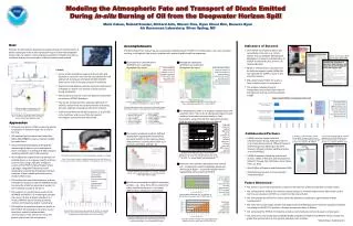
Total Gaseous Mercury (ng/m3) at Neuglobsow: June 26 – July 6, 1995 measurements 24
Total Particulate Mercury (pg/m3) at Neuglobsow, Nov 1-14, 1999 measurements 25
EMEP Intercomparison Study of Numerical Models for Long-Range Atmospheric Transport of Mercury Intro-duction Stage I Stage II Stage III Conclu-sions Chemistry Hg0 Hg(p) RGM Wet Dep Dry Dep Budgets Reactive Gaseous Mercury at Neuglobsow, Nov 1-14, 1999 26
atmospheric chemistry inter-converts mercury forms Hg(0) Hg from other sources: local, regional & more distant Hg(II) Hg(p) atmospheric deposition to the water surface emissions of Hg(0), Hg(II), Hg(p) atmospheric deposition to the watershed Measurement of ambient air concentrations Measurement of wet deposition AMBIENT AIR CONCENTRATIONS • more fundamental – easier to diagnose • need continuous – episodic source impacts • need speciation – at least RGM, Hg(p), Hg(0) • need data at surface and above WET DEPOSITION • complex – hard to diagnose • weekly – many events • background – also need near-field 29
Hg from other sources: local, regional & more distant atmospheric deposition to the water surface atmospheric deposition to the watershed Measurement of ambient air concentrations Measurement of wet deposition 30
Example of results: Rock Creek Watershed 32
Largest Model-Estimated U.S./Canada Anthropogenic Contributors to 1999 Mercury Deposition to the Rock Creek Watershed (large region) 33
Largest Model-Estimated U.S./Canada Anthropogenic Contributors to 1999 Mercury Deposition to the Rock Creek Watershed (close up) 34
Proportions of 1999 Model-Estimated AtmosphericDeposition to the Rock Creek Watershed from DifferentAnthropogenic U.S./Canada Mercury Emissions Source Sectors 35
Top 25 Contributors to Hg Deposition to Rock Creek Watershed 36
Atmospheric Deposition Flux to the Rock Creek Watershedfrom Anthropogenic Mercury Emissions Sources in the U.S. and Canada 37
Thanks! For more information on this research: http://www.arl.noaa.gov/ss/transport/cohen.html 38 38
Extra Slides
Hg from other sources: local, regional & more distant atmospheric deposition to the water surface emissions of Hg(0), Hg(II), Hg(p) atmospheric deposition to the watershed 42
Elemental Mercury [Hg(0)] Upper atmospheric halogen-mediated heterogeneous oxidation? Polar sunrise “mercury depletion events” Hg(II), ionic mercury, RGM Particulate Mercury [Hg(p)] Br cloud CLOUD DROPLET Hg(II) reducedto Hg(0) by SO2 and sunlight Vapor phase: Hg(0) oxidized to RGM and Hg(p) by O3, H202, Cl2, OH, HCl Adsorption/ desorption of Hg(II) to /from soot Hg(p) Primary Anthropogenic Emissions Hg(0) oxidized to dissolved Hg(II) species by O3, OH, HOCl, OCl- Wet deposition Dry deposition Re-emission of previously deposited anthropogenic and natural mercury Natural emissions Atmospheric Mercury Fate Processes 43
policy development requires: • source-attribution (source-receptor info) • estimated impacts of alternative future scenarios • estimation of source-attribution & future impacts requires atmospheric models • atmospheric models require: • knowledge of atmospheric chemistry & fate • emissions data • ambient data for “ground-truthing”
Atmospheric Mercury Model Meteorology Transport and Dispersion Atmospheric Chemistry Wet and Dry Deposition Emissions Model results Source attribution Model evaluation Measurements at specific locations Ambient concentrations and deposition
Some Current Atmospheric Chemistry Challenges • Plume chemistry, e.g., rapid reduction of RGM to elemental mercury? • If significant reduction of RGM to Hg(0) is occurring in power-plant plumes, then much less local/regional deposition 47
RGM reduction in power-plant plumes? • If significant reduction of RGM to Hg(0) is occurring in power-plant plumes, then much less local/regional deposition • No known chemical reaction is capable of causing significant reduction of RGM in plumes – e.g. measured rates of SO2 reduction can’t explain some of the claimed reduction rates • Very hard to measure • Aircraft • Static Plume Dilution Chambers (SPDC) • Ground-based measurements 48
RGM reduction in power-plant plumes? • Most current state-of-the-science models do not include processes that lead to significant reduction in plumes • Recent measurement results show less reduction • Significant uncertainties – e.g., mass balance errors comparable to measured effects… • Current status – inconclusive… but weight of evidence suggest that while some reduction may be occurring, it may be only a relatively small amount • Recent measurements at Steubenville, OH appear to show strong local mercury deposition from coal-fired power plant emissions. 49
Some Current Atmospheric Chemistry Challenges • Plume chemistry, e.g., rapid reduction of RGM to elemental mercury? • Boundary conditions for regional models? 50