
Evolutionary Sequence Models: Understanding HIV Pol Sequences
E N D
Presentation Transcript
JC69: Jukes-Cantor (1969) Model Assumes all bases interchange with equal probabilities, equal base frequencies
F81: Felsenstein (1981) Model Assumes all bases interchange with equal probabilities, base frequencies may vary.
HKY85: Hasegawa, Kishino, Yano (1985) Model Assumes unequal transition and transversion probabilities, base frequencies may vary.
REV: General Time Reversible Model Assumes unequal probabilities for all substitution types, base frequencies may vary.
Other Forms of Rate Heterogeneity • Variation from gene to gene • Variation from site to site within a gene • Synonymous vs synonymous rates • Spatial rate heterogeneity • Variation from lineage to lineage • Correlations among sets of sites
Gamma models of site-to-site heterogeneity • Hierarchical model: • Evolutionary rates at individual sites are drawn from a gamma distribution • Given the rate at a particular site, sequence evolution follows one of the previously discussed models • Original idea: Uzzel and Corbin (1971) • First likelihood treatment was by Yang (1993)
REV+G: General Time Reversible Model with Gamma Rate Heterogeneity (Yang 1993)
“All” we are doing here is integrating the likelihood function over all possible rate values, with those values being weighted according to probabilities assigned by the gamma distribution.
Calculating the integral in the continuous case is very expensive. • Yang (1994) suggested “discretizing” the gamma distribution, and using the discrete form of the likelihood function. • The cost of calculation increases only linearly with the number of rate categories, N.
Correlations among sites • Codons • Dinucleotides (secondary structure) General idea: move from 4-state nucleotide models to 16- or 64-state models.
This approach can be combined with any nucleotide model • Rate heterogeneity can be added in the same way as with nucleotide models • Account for correlations among nucleotide sites within codons • Avoids the problematic notion of “degeneracy classes” • Necessary for rigorous estimates of synonymous and nonsynonymous substitution rates.
Consider the result of allowing gamma variation in rates over codons: • While they are allowed to have different magnitudes, the two classes of rates have the same distribution. • Synonymous rates are likely to be less variable over sites than are nonsynonymous rates.
Site-to-site rate variation, transitions and transversions with independent distributions A C G T A C G T
Each site in the sequence has a (random) synonymous rate, and a (random) nonsynonymous rate, drawn from some bivariate distribution, The likelihood is again integrated with respect to f:
As before, the likelihood function is discretized for computational feasibility: The discretization process can be tricky in general. In all that follows, we assume that are independent gamma random variables, which allows discretization of each axis separately.
Goals of molecular evolutionary analyses • Understand the structure of • Are parameter values (i.e., rates) equal among different branches? • Is the structure of (e.g., TS/TV ratio) the same for different branches? • Are the values of such parameters “related” among different genes?
B A G Likelihood function for homologous DNA sequences x is the collection of all parameters affecting the evolution of sequences A, B, and G. is the collection of all data (sequences A, B, and G).
Relative Rate Tests Are evolutionary rates the same along two lineages? B A G
Versions of the relative rate test • Distance based (Wu and Li 1985) • For 2 clades (Li and Bousquet 1992) • Likelihood ratio (Muse and Weir 1992) • Nonparametric (Tajima 1993)
B A G Likelihood-based RR Test • Maximize L assuming • Maximize L without constraints • LRT has a chi-squared distribution if rates are equal Note: Use of outgroup insures that the unknown divergence time is irrelevant.
g b a B A G Distance-based RR Tests
B A G Nonparametric RR Test
ndhF rbcL Nonsyn Syn
Locus A Locus B Locus effect Lineage effect Lineage X Locus effect
Relative Ratio Tests • Are “branch lengths” proportional among loci? • Muse and Gaut 1997; Muse et al. 1997; Huelsenbeck et al. 1997; Yang 1995
1 1 2 2 3 3 4 4 Relative Ratio Test The null hypothesis is that the relative proportions of branch lengths are the same for all loci. The proportion need not be known a priori.