Download
1 / 17
170 likes | 349 Vues
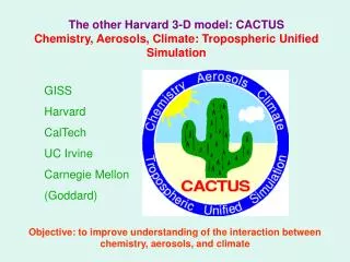
The other Harvard 3-D model: CACTUS Chemistry, Aerosols, Climate: Tropospheric Unified Simulation. GISS Harvard CalTech UC Irvine Carnegie Mellon (Goddard). Objective: to improve understanding of the interaction between chemistry, aerosols, and climate. Anatomy of a Unified Model.

E N D
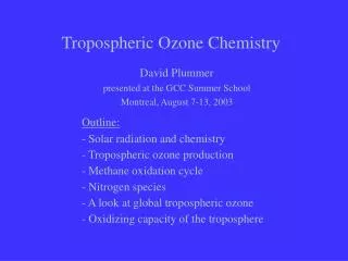
The other Harvard 3-D model:CACTUSChemistry, Aerosols, Climate: Tropospheric Unified Simulation GISS Harvard CalTech UC Irvine Carnegie Mellon (Goddard) Objective: to improve understanding of the interaction between chemistry, aerosols, and climate
Anatomy of a Unified Model GHG concentrations, solar flux, land surface characteristics GISS GCM II’ calculates meteorology aerosol tropospheric ozone temperature, humidity, wet dep, clouds, winds, etc CalTech aerosol module Harvard chemistry module aerosol, gases precursor emissions
What follows: Alternative, practical approaches, with tie-in to GEOS CHEM Fully coupling a model is ambitious and CPU-intensive! (wallclock time: 10 days/model year) Equilibrium climate simulations: 75-100 years, including spin-up Transient simulations: 50 years just for ocean spin-up
Chapter 1: Calculate radiative forcing due to increase in tropospheric ozone (Mickley et al., 1999, 2001) GHG concentrations, solar flux, land surface characteristics GISS GCM II’ Forcing calculation ozone Calculated ozone does not influence climate meteorology Harvard chemistry module Specified aerosol. Present-day & preindustrial precursor emissions (run twice)
Uncertainty of radiative forcing due to O3 is quite large. Standard simulation, DF = 0.44 Wm-2 Test simulation with natural emissions within range of uncertainty DF = 0.80 Wm-2 (about 1/2 DF of CO2) std model test model obs, late 1800s Preindustrial ozone monthly means Mickley et al., 2001
Chapter 1 continued: Do same forcing calculation for sulfate aerosol (Adams et al., 1999) GHG concentrations, solar flux, land surface characteristics Forcing calculation GISS GCM II’ aerosol meteorology CalTech aerosol module Harvard offline chemistry nitric acid precursor emissions
Nitrate forcing may have large impact over 21st century DF preindustrial to present-day for sulfate+nitrate = -1.14 Wm-2 DF preindustrial to 2100 for sulfate+nitrate = -2.13 Wm-2 Adams et al., 2001 2100 annual averaged forcing due to sulfate+nitrate aerosol
Chapter 2: Begin to unify model (Liao et al., 2003) GHG concentrations, solar flux, land surface characteristics Forcing calculation Forcing calculation GISS GCM II’ aerosol ozone meteorology CalTech aerosol module Harvard chemistry module oxidants, nitric acid precursor emissions
Heterogeneous chemistry decreases ozone at the surface Ratio of annual mean mixing ratios of ozone: With het chem / without hem chem Includes ozone uptake on mineral dust. Liao et al., 2003
Chapter 3: Calculate equilibrium climate response to changing tropospheric ozone (Mickley et al., 2003) GHG concentrations, solar flux, land surface characteristics GISS GCM II’ calculates meteorology archived monthly mean ozone fields Calculate preindustrial and present-day ozone fields beforehand, using present-day climate. Harvard chemistry module precursor emissions
Results from GCM equilibrium simulation with present-day vs. preindustrial tropospheric ozone equilibrium climate DF = 0.49 W m-2 Present-day ozone DT = 0.3oC Preindustrial ozone Mickley et al., 2003
Inhomogeneity of climate response to tropospheric ozone change over 20th century • Greater warming in northern hemisphere (due to more ozone and albedo feedback in Arctic) • Strong cooling in stratosphere (>1oC in Arctic winter): Global NH Stratospheric ozone SH Tropospheric ozone 9.6 mm Surface
Chapter 3 continued (Chung et al., in progress) Do same with Caltech aerosol: Feed monthly mean preindustrial and present-day aerosol fields into GISS GCM.
Chapter 4: Build interface between GISS GCM and GEOS CHEM to study past and future climates GHG concentrations, solar flux, land surface characteristics GISS GCM II’ archived temperatures, humidity, winds, etc First application: investigate effect of future climate change on US air quality (Mickley, Shiliang Wu) GEOS CHEM calculates chemistry, aerosol precursor emissions
Chapter 4 continued: Diagnose effect of changing climate on US air quality (transient simulation) GISS GCM, with changing GHGs 1950 2000 2025 2050 2075 2100 Spin-up of ocean archived temperatures, humidity, winds, etc GEOS-CHEM Calculate chemistry, aerosol present-day precursor emissions
Chapter 5: Investigate effect of aerosol and tropospheric ozone on future climate GISS GCM, with changing GHGs + ozone, aerosol 1950 2000 2025 2050 2075 2100 Spin-up of ocean archived temperatures, humidity, winds, etc GEOS-CHEM Calculate chemistry, aerosol precursor emissions Develop 100-year forecast of ozone, aerosol 1950 2000 2025 2050 2075 2100
Chapter 6: Investigate indirect effect of aerosols (Adams, DelGenio) Acknowledgments: Brendan Field, David Rind, Jean Lerner, Reto Ruedy, Gavin Schmidt, Drew Shindell, Andy Lacis, Prashant Murti, Bob Yantosca