Download

1 / 16
170 likes | 383 Vues
Household Production and Life-Cycle and Labor Supply. Household Production. As in the study of labor demand, we can alter the variables to explore the impacts of utility maximization and the accompanying income and substitution effects of labor supply.

E N D
Household Production • As in the study of labor demand, we can alter the variables to explore the impacts of utility maximization and the accompanying income and substitution effects of labor supply. • In the previous analysis, we ignored household production. Household production of goods and services is an alternative to participation in the labor force and purchased goods and services that flow from that participation.
Assumptions • Two alternatives: Purchased goods and services that come from working for pay and home produced goods and services that come from hours spent at home. • Hours spent at home are directly related to home produced goods. • Assume that leisure is zero • Single decision-maker • Household does not save or borrow
Graphical Model • Value of purchased goods and services on Y axis and hours spend at home on the X axis (proxies value of home production) • Hours spent at home = 16 hours - Hours spent working for pay • Hh = 16 – H • Value of purchased goods and services is equal to Y = W x H • Constraint is similar to previous model with a slope of -W • Indifference curves or utility isoquants assume that home produced goods (GS) and services and substitutes for purchased goods and services (Hh) • The utility isoquants are convex reflecting that: • High GS and low Hh : ΔGS/ΔHh is high or isoquant is steeper • Low GS and high Hh : ΔGS/ΔHh is low or isoquant is flatter
Ray from the origin reflects ration of GS to Hh • If GS/Hh is high, ΔGS/ΔHh is also relatively high. When you an extra hour of Hh one has to give up a lot of purchased goods and services to remain equally well off. Why? At low levels of Hh time spend at home is more highly valued relative to GS. • If GS/Hh is low, ΔGS/ΔHh is also relatively low. When you an extra hour of Hh one has to give up only a few purchased goods and services to remain equally well off. Why? At high levels of Hh time spend at home is less highly valued relative to GS. • Work preferrer has a flatter isoquant. • Home preferrer has a steeper isoquant.
Changes in Wages • Changes in wages changes the “income/wage” constraint and produces income and substitution effects. • The choice between time spent in the household and the time spent at work depends upon income and substitution effects • The observed increases in participation rate of women and the convergence of participation rates with men indicates that the substitution effect has outweighed the income effect but the relatively strength of the substitution effect has been diminishing as participation rates approach those of men.
Tripartite Choice • The analysis can be expanded by including the labor-leisure choice. Households must decide between time at work, time in household production and time spent in leisure. • Two income and substitution effects as wages change. For example, as wages rise, • Substitute time in household for time at work • Initially, time at household can more easily be given up through labor-saving devices and childcare. However, as participation rates and hours worked of breadwinners rises, this becomes more difficult. • Substitute leisure for time at work • Leisure activities usually require time so it is more difficult to substitute for them • This may explain the initial rapid increase in participation and hours worked and why the trend is diminishing.
Figure 7.2Large versus Small Substitution Effects Attendant to a Wage Increase
Joint Labor Supply Decisions • Dropping the assumption of one decision-maker, economists have looked at models of joint labor supply: • Retain single decision-maker either home dictator or identical preferences. • Bargaining process with resources determining bargaining power. • Act independently, but consider the impacts of their actions on the other party.
Specialization: household utility maximization with different productivities. • Productivity in work place • Productivity at home (household productivity and satisfaction from child-rearing). • Some studies demonstrate the division of housework depends on the relative wage • Many households maximize utility with both individuals working. See graph. • Cross effects: Spouse’s decision to work more for pay affects the other spouse household productivity in production or consumption. • If spouses are substitutes in household production, if one spouse works more the other may become more productive and increase the amount of time they stay at home. If they are complements, the other may work more. • If spouses are complements in consumption, the other may work more. Substitutes in consumption reflect a problematic marriage so…
Household Productivity in Recessions • Recession causes spouse to become unemployed: • The unemployed workers productivity at work drops and the opportunity cost of working at home goes down. • The relative productivity of the worker’s spouse rises if their potential wages do not change. • Substitute unemployed worker for spouse’s participation in household production and the spouse goes to work. • As family income falls, less goods and services and less leisure time are demanded. • This creates an “additional worker” effect.
On the other hand, the expected wage of either spouse may have also fallen. • Decreases in expected wages create a substitution effect towards less work and more leisure. • This would tend to create a “discouraged worker” effect. • Discouraged and part-time workers are part of “hidden” unemployment.
Life Cycle Aspects • Dynamic preferences or labor productivity at home and changing labor participation patterns • Presence of young children can make an indifference curve steeper and the absence of younger children make the indifference curve flatter. • Presence of a disabled child, parent or spouse.