Download
1 / 39
390 likes | 549 Vues
This paper presents an innovative isotropic material remap scheme for Eulerian codes, specifically developed within the CTH framework at Sandia National Laboratories. The remap strategy addresses key challenges in computational hydrodynamics, allowing for efficient simulation of complex material interactions during dynamic events. The methodology encompasses detailed explanations of the conservation equations, adaptive mesh refinement, and the interface reconstruction process. Results from various high-performance computing platforms demonstrate the robustness and scalability of the approach in real-world applications.

E N D
An Isotropic Material Remap Scheme for Eulerian Codes Raymond L. Bell Computational Shock and Multi-Physics Department Sandia National Laboratories Albuquerque, NM 87185 Presented at the: 2nd International Conference on Cybernetics and Information Technologies, Systems and Applications (CITSA 2005) jointly with the 11th International Conference on Information Systems Analysis and Synthesis (ISAS 2005) July 14-17, 2005 - Orlando, Florida, USA Sandia is a multiprogram laboratory operated by Sandia Corporation, a Lockheed Martin Company,for the United States Department of Energy under contract DE-AC04-94AL85000.
Outline • Code Description • CTH Definition • Equations Solved • Computer platforms • Solution Sequence • CTH Code Family • Equations of State and Constitutive Models • Adaptive Mesh Refinement (AMR) • Material Interface Reconstruction • Isotropic Material Remap Option • Motivation • Interface Reconstruction • Conclusion
Code Description • CTH has been under development and in use for several decades. • 1D, 2D, and 3D explicit Eulerian Code • Direct Descendant of CSQ (a 2D Eulerian Code) • CSQ Evolved from the 1D Lagrangian Code known as CHART-D (Combined Hydro and Radiation Transport Diffusion) • To get the acronyms out of the way: • CSQ = [CHART-D] 2 • CTH = [CSQ]3/2 = [CHART-D]3 • Licensed to over 340 institutions, most are DOE Laboratories, DoD Laboratories, or DoD/DOE affiliated contractors.
Some Typical CTH Problems Projectile Impact Test Simulation
Equations Solved Conservation of mass Conservation of momentum Conservation of energy Where: ρ = mass density This set of coupled partial differential V = velocity vector equations is numerically solved on a fixed σ = stress tensor Eulerian Mesh using Equations of State to Q = artificial viscosity close the system. P = cell pressure E = specific energy F = applied body force S = energy source term
Computer Platforms • Initially CTH was targeted for CRAY super computers. • CTH was highly ‘vectorized’. • Current super computers are massively parallel, uses Message Passing Interface (MPI) algorithms. • CTH scales quite nicely on “single instruction multiple data” (SIMD) platforms. • CTH is routinely run on virtually any platform available from massively parallel supercomputers, to Linux clusters, to laptops running windows. • Calculations containing more than a billion cells have been run on SNL massively parallel computers.
CTH Solution Sequence • Many explicit Eulerian codes integrate the conservation equations through time in a two-step process • Lagrangian step, in which the computational mesh distorts to follow motion of the materials • Remap step, in which the mesh is remapped back onto the original mesh
CTH Solution Sequence • Adaptive Mesh Refinement update (if AMR calc.) • Refinement, if needed, every 2-3 cycles • Unrefinement, if needed, every 6 cycles • Lagrangian Step • Lagrangian forms of conservation equations are solved for time step • Remap Step • Distorted mesh is mapped onto the original mesh • Database Modification Step • Database is modified based on user directives • e.g. Discard, Velocity addition, etc. • Time Step Control
Eulerian and Lagrangian Definitions • EULERIAN - Treatment of a continuum variable (i.e., temperature) from a fixed frame of reference. Equations of motion and conservation are solved using a mesh fixed in space so that material moves relative to the mesh. • LAGRANGIAN - Treatment of a continuum variable (i.e., temperature) from a frame of reference fixed with respect to the material. Equations of motion and conservation are solved using a mesh fixed with respect to the material so that the mesh moves through space.
Mesh and Computational Cell • Mesh is Generated From 3 Sets of Spatial Coordinates • {xi},{ yj}, {zk} define cell boundaries • Each cell is a rectangular parallelepiped (box) • Spatial & Temporal Positions • Most variables are cell centered and defined at the time step • Velocities are on and normal to the cell face and half time step centered Vz P, T, ... Vx Vy
Half Index Shifted Momenta • During the remap step, the velocity values at each face are assigned to each of the cell centers (for the cells sharing the face) • These cell centered momenta (velocity multiplied by the mass in the cell) are advected with the total mass moving over the cell boundaries. • New face centered velocity is defined as the sum of the residual cell centered momenta (one orange and one green value) divided by the sum of the updated masses in the 2 cells sharing the face.
Cell Thermodynamics Update • After the remap step is completed, new material pressures, temperatures, and sound speeds are determined (EOS). • Cell average pressure, average temperature, and average sound speed are also determined using MMP options. • MMP0 (default) uses volume fraction weighted pressure and heat capacity weighted temperature. • MMP2 uses material compressibility as a weighting factor for cell pressure. • All options use volume fraction weighted sound speed.
Database Modification Step DATABASE IS MODIFIED BASED ON USER DIRECTIVES • User may modify database in a variety of ways • Rigid mesh velocity - User may add constant velocity field to a specified region of the mesh at specified times • Discard material • within user-specified range of pressure, density, temperature, energy, and volume fraction
Time Step Control • Next time step is computed based on Courant stability criteria • Solution for a cycle is complete at conclusion of Timestep Control
Restart and Plot Files Periodic Restart and Plot Files are written as directed by the user • Restart Files contain all data necessary to restart a calculation at a given problem time. • Plot Files contain truncated information designated by the user as information that will be plotted at the end of the calculation. • Not sufficient for restarting a calculation. • Only those variables that are to be plotted.
CTH Code Family • Code family consists of seven major codes • CTHGEN - generates initial database (deprecated) • CTH - integrates problem through time • CTHED - text processing • CTHREZ - manual rezoner • CTHPLT - graphics post processing • SPYMASTER (SPYPLT) - on the fly or post processing graphics • HISPLT - history graphics post processing • Software mostly written in ANSI FORTRAN 77 with some C
CTH Equations-of-State • Mie-Grüneisen analytic formula, including porosity • SESAME tabular option, including porosity • Jones-Wilkins-Lee analytic formula (including programmed burn) for High Explosive (HE) materials • Ideal gas analytic formula • Brittle Material EOS’s • Geological Material EOS’s
CTH Constitutive Models Material Strength Models • Elastic/Perfectly-Plastic • von Mises and pressure dependent yield surfaces • Thermal softening and density degradation • Johnson-Cook • Other Advanced Constitutive Models include Brittle Material (ceramic, concrete, etc) response
Adaptive Mesh Refinement • Adaptive Mesh Refinement (AMR) utilizes a ‘patch’ block based scheme (available on single and multi-processor platforms). • All AMR blocks are logically identical (same number of cells in the same configuration). • Each block differs is in cell sizes and the coordinates of the volume being discritized. • Adjacent blocks may contain cells that are identical, 1/2 the size, or twice the size compared to their neighbor block cells. • User defined ‘refinement indicators’ determine which portions of the problem space are refined.
Interface Tracking Algorithms • Advection volumes are calculated using t(n+1/2) velocities. • Reconstruction techniques determine material interfaces. • Simple Line Interface Construction (SLIC) Algorithm • Considers presence of materials in cell behind and ahead of donor • Algorithm has well-known biases • High Resolution Interface Tracking (HRIT) Algorithm • Considers presence of materials in all neighbor cells • HRIT algorithm available only for 2D • Sandia Modified Youngs’ Reconstruction Algorithm (SMYRA) • Considers presence of materials in all neighbor cells • Gives best results in 3D and identical results to HRIT in 2D
Advection Volumes mat 2 mat 1 Interface Tracking Algorithms
Interface Tracking Benchmark Problem Starting Conditions
The Isotropic Remap Option • Motivation: • Difficulties encountered when advecting multi-phase materials • Original scheme: • sum volume fractions, masses, and energies for the parent and child materials into the parent material locations. • zero child values. • required extra variables describing the ‘child to total’ ratios. • interface tracking algorithm works on all materials but the child. • child and parent values recovered using the advected extra variable values. • Method required several extra variables and was not easily extended to other mixtures (gas mixtures, etc.).
The Isotropic Remap Option • Interface Reconstruction: • In calculations with materials that are somehow thoroughly mixed (multiphase materials or a gas mixture for instance), no interface should exist between these materials. • Users may define groups of materials that should be kept together. • This option will define an interface between groups of materials • - all materials will be assigned to a group • - some groups will contain only one material • In a multi-material group, the group volume fraction is the sum of the volume fractions of the group members. • In a single material group it is the volume fraction for that material.
The Isotropic Remap Option • Group Advection: • Advection volumes are calculated using the cell face centered velocities. • Advection volumes are then sub-divided by groups (rather than by material) using the interface reconstruction algorithms. • Advection volume for each member material is determined by the relative volume fractions of the group member materials in the donor cell. • The advection step is then completed as usual.
(a) Before Group Summation Group 1 Group 2 (b) After Group Summation The Isotropic Remap Option Group 1: Blue material Orange Material Group 2: Green Material (c) After Advection and Group Division
The Isotropic Remap Option Illustration: Grouped advection Un-Grouped Advection Inner lower ring is 33% material 1 and 67% material 3, 4 zones across the thickness Note how regular interface scheme tries to separate materials 1 and 3 Material 1 is blue, 2 is gold, and 3 is red (in mixed cells, most abundant material is plotted)
The Isotropic Remap Option Illustration: Un-Grouped Advection Grouped advection Grouped advection maintains original concentrations Un-Grouped advection results in Materials being separated and the concentrations increased
Conclusion • By creating this isotropic remap option, we have eliminated some of the previously required extra variables for multi-phase materials and allowed an easily used capability for defining groups of materials that should not be separated (mixed materials such as dusty gases or gas mixtures) during the advection step. • I want to thank Dr David Crawford (CTH Development Team Lead) and Dr Robert Schmitt, both of SNL Department 9116, for providing me the opportunity to create this algorithm along with some of the materials I have used in my paper and this presentation.