
VI Function Evaluation
VI Function Evaluation. Learn hardware algorithms for evaluating useful functions Divisionlike square-rooting algorithms Evaluating sin x , tanh x , ln x , . . . by series expansion Function evaluation via convergence computation

VI Function Evaluation
E N D
Presentation Transcript
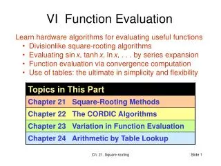
VI Function Evaluation • Learn hardware algorithms for evaluating useful functions • Divisionlike square-rooting algorithms • Evaluating sinx, tanhx, lnx, . . . by series expansion • Function evaluation via convergence computation • Use of tables: the ultimate in simplicity and flexibility Ch. 21. Square-rooting
21 Square-Rooting Methods Chapter Goals Learning algorithms and implementations for both digit-at-a-time and convergence square-rooting Chapter Highlights Square-rooting part of ANSI/IEEE standard Digit-recurrence (divisionlike) algorithms Convergence or iterative schemes Square-rooting not special case of division Ch. 21. Square-rooting
Square-Rooting Methods: Topics Ch. 21. Square-rooting
Fig. 21.3 Binary square-rooting in dot notation. 21.1 The Pencil-and-Paper Algorithm Notation for our discussion of division algorithms: z Radicand z2k–1z2k–2 . . . z3z2z1z0 q Square root qk–1qk–2 . . . q1q0 s Remainder, z – q2sksk–1sk–2 . . . s1s0 Remainder range, 0 s 2q (k + 1 digits) Justification: s 2q + 1 would lead to z = q2 + s (q + 1)2 Ch. 21. Square-rooting
Root digit Partial root q2q1q0qq(0) = 0 9 5 2 4 1 zq2 = 3 q(1) = 3 9 0 5 2 6q1q1 52 q1 = 0 q(2) = 30 0 0 5 2 4 1 60q0q0 5241 q0 = 8 q(3) = 308 4 8 6 4 0 3 7 7 s = (377)tenq = (308)ten “sixty plus q1” Example of Decimal Square-Rooting1 Check: 3082 + 377 = 94,864 + 377 = 95,241 Fig. 21.1 Extracting the square root of a decimal integer using the pencil-and-paper algorithm. Ch. 21. Square-rooting
Example of Decimal Square-Rooting2 308 3 9 5 2 4 1 3 9 ------ 6 0 0 5 2 0 0 0 --------- 6 0 8 5 2 4 1 8 4 8 6 4 ------------- 0 3 7 7 Ch. 21. Square-rooting
Example of Decimal Square-Rooting3 312 = 961 q2 = 3, q1 =1 (q2*10+q1)2 =(q2*10)2+2q2*q1*10+q12 = (q2*10)2+(2q2*10+q1)q1 312 3 9 7 5 4 1 3 9 ------ 6 1 0 7 5 1 6 1 --------- 6 2 2 1 4 4 1 2 1 2 4 4 ------------- 0 1 9 7 (q2*10)2 (2q2*10+q1)= 61 q1=1 (2q2*10+q1)q1= 61 Ch. 21. Square-rooting
Root Digit Selection Rule The root thus far is denoted by q(i) = (qk–1qk–2 . . . qk–i)ten Attaching the next digit qk–i–1, partial root becomes q(i+1) = 10q(i) + qk–i–1 The square of q(i+1) is 100(q(i))2 + 20q(i)qk–i–1 + (qk–i–1)2 100(q(i))2 = (10q(i))2 subtracted from partial remainder in previous steps Must subtract (10(2q(i) + qk–i–1) qk–i–1 to get the new partial remainder More generally, in radix r, must subtract (r(2q(i)) + qk–i–1) qk–i–1 In radix 2, must subtract (4q(i) + qk–i–1) qk–i–1, which is 4q(i) + 1 for qk–i–1 = 1, and 0 otherwise Thus, we use (qk–1qk–2 . . . qk–I 0 1)two in a trial subtraction Ch. 21. Square-rooting
Example of Binary Square-Rooting Check: 102 + 18 = 118 = (0111 0110)two Root digit Partial root q3 q2q1q0qq(0) = 0 0 11 10 11 0 01? Yesq3 = 1 q(1) = 1 0 1 0 0 1 1 101? No q2 = 0 q(2) = 10 0 0 0 0 1 1 0 1 1001? Yes q1 = 1 q(3) = 101 1 0 0 1 0 1 0 0 1 0 10101? No q0 = 0 q(4) = 1010 0 0 0 0 0 1 0 0 1 0 s = (18)tenq=(1010)two=(10)ten Fig. 21.2 Extracting the square root of a binary integer using the pencil-and-paper algorithm. Ch. 21. Square-rooting
Example of Binary Square-Rooting Check: 102 + 18 = 118 = (0111 0110)two 1010q 0 11 10 11 0 01? Yesq3 = 1 0 1 0 0 1 1 101? No q2 = 0 0 0 0 0 1 1 0 1 1001? Yes q1 = 1 1 0 0 1 0 1 0 0 1 0 10101? No q0 = 0 0 0 0 0 0 1 0 0 1 0 1 1 1 0 0 0 -------------- 1 0 0 1 1 -------------- 1 0 1 0 0 0 Fig. 21.2 Extracting the square root of a binary integer using the pencil-and-paper algorithm. Ch. 21. Square-rooting
21.2 Restoring Shift/Subtract Algorithm Consistent with the ANSI/IEEE floating-point standard, we formulate our algorithms for a radicand in the range 1 z < 4 (after possible 1-bit shift for an odd exponent) 1 z < 4 Radicand z1z0 .z–1z–2. . . z–l 1 q < 2 Square root 1 .q–1q–2 . . . q–l 0 s < 4 Remainder s1s0 .s–1s–2. . .s–l Binary square-rooting is defined by the recurrence s(j) = 2s(j–1) – q–j(2q(j–1) + 2–jq–j) with s(0) = z – 1, q(0) = 1, s(j) = s where q(j) is the root up to its (–j)th digit; thus q = q(l) To choose the next root digit q–j {0, 1}, subtract from 2s(j–1) the value 2q(j–1) + 2–j = (1q-1(j–1).q-2(j–1). . . q-j+1(j–1)0 1)two A negative trial difference means q–j = 0 Ch. 21. Square-rooting
Root digit Partial root ================================ z (radicand = 118/64) 0 1 . 0 1 0 1 1 0 ================================ s(0) = z – 1 0 0 0 . 1 1 0 1 1 0 q0 = 1 1. 2s(0) 0 0 1 . 1 0 1 1 0 0 –[2 (1.)+2–1] 1 0 . 1 ––––––––––––––––––––––––––––––––– s(1) 1 1 1 . 0 0 1 1 0 0 q–1 = 0 1.0 s(1) = 2s(0)Restore 0 0 1 . 1 0 1 1 0 0 2s(1) 0 1 1 . 0 1 1 0 0 0 –[2 (1.0)+2–2] 1 0 . 0 1 ––––––––––––––––––––––––––––––––– s(2) 0 0 1 . 0 0 1 0 0 0 q–2 = 1 1.01 2s(2) 0 1 0 . 0 1 0 0 0 0 –[2 (1.01)+2–3] 1 0 . 1 0 1 ––––––––––––––––––––––––––––––––– s(3) 1 1 1 . 1 0 1 0 0 0 q–3 = 0 1.010 s(3) = 2s(2)Restore 0 1 0 . 0 1 0 0 0 0 2s(3) 1 0 0 . 1 0 0 0 0 0 –[2 (1.010)+2–4] 1 0 . 1 0 0 1 ––––––––––––––––––––––––––––––––– s(4) 0 0 1 . 1 1 1 1 0 0 q–4 = 1 1.0101 2s(4) 0 1 1 . 1 1 1 0 0 0 –[2 (1.0101)+2–5] 1 0 . 1 0 1 0 1 ––––––––––––––––––––––––––––––––– s(5) 0 0 1 . 0 0 1 1 1 0 q–5 = 1 1.01011 2s(5) 0 1 0 . 0 1 1 1 0 0 –[2(1.01011)+2–6] 1 0 . 1 0 1 1 0 1 ––––––––––––––––––––––––––––––––– s(6) 1 1 1 . 1 0 1 1 1 1 q–6 = 0 1.010110 s(6) = 2s(5)Restore 0 1 0 . 0 1 1 1 0 0 s (remainder = 156/64) 0 . 0 0 0 0 1 0 0 1 1 1 0 0 q (root = 86/64) 1 . 0 1 0 1 1 0 ================================ Finding the Sq. Root of z = 1.110110 via the Restoring Algorithm Fig. 21.4Example of sequential binary square-rooting using the restoring algorithm. q–7 = 1, so round up Ch. 21. Square-rooting
Fig. 13.5 Shift/subtract sequential restoring divider (for comparison). Hardware for Restoring Square-Rooting Fig. 21.5 Sequential shift/subtract restoring square-rooter. Ch. 21. Square-rooting
Rounding the Square Root In fractional square-rooting, the remainder is not needed To round the result, we can produce an extra digit q–l–1: Truncate for q–l–1 = 0, round up for q–l–1 = 1 Midway case, q–l–1=1 followed by all 0s, impossible (Prob. 21.11) Example: In Fig. 21.4, we had (01.110110)two = (1.010110)two2 + (10.011100)/64 An extra iteration produces q–7 = 1 So the root is rounded up to q = (1.010111)two = 87/64 The rounded-up value is closer to the root than the truncated version Original: 118/64 = (86/64)2 + 156/(64)2 Rounded: 118/64 = (87/64)2 – 17/(64)2 Ch. 21. Square-rooting
Slight complication, compared with nonrestoring division This term cannot be formed by concatenation 21.3 Binary Nonrestoring Algorithm As in nonrestoring division, nonrestoring square-rooting implies: Root digits in {-1, 1} On-the-fly conversion to binary Possible final correction The case q–j = 1 (nonnegative partial remainder), is handled as in the restoring algorithm; i.e., it leads to the trial subtraction of q–j [2q(j–1) + 2–jq–j ] = 2q(j–1) + 2–j For q–j = -1, we must subtract q–j [2q(j–1) + 2–jq–j ] = –[2q(j–1) – 2–j] which is equivalent to adding 2q(j–1) – 2–j Ch. 21. Square-rooting
================================ z (radicand = 118/64) 0 1 . 1 1 0 1 1 0 ================================ s(0) = z – 1 0 0 0 . 1 1 0 1 1 0 q0 = 1 1. 2s(0) 0 0 1 . 1 0 1 1 0 0 q–1 = 1 1.1 –[2 (1.)+2–1] 1 0 . 1 ––––––––––––––––––––––––––––––––– s(1) 1 1 1 . 0 0 1 1 0 0 q–2 = -1 1.01 2s(1) 1 1 0 . 0 1 1 0 0 0 +[2 (1.1)-2–2] 1 0 . 1 1 ––––––––––––––––––––––––––––––––– s(2) 0 0 1 . 0 0 1 0 0 0 q–3 = 1 1.011 2s(2) 0 1 0 . 0 1 0 0 0 0 –[2 (1.01)+2–3] 1 0 . 1 0 1 ––––––––––––––––––––––––––––––––– s(3) 1 1 1 . 1 0 1 0 0 0 q–4 = -1 1.0101 2s(3) 1 1 1 . 0 1 0 0 0 0 +[2 (1.011)-2–4] 1 0 . 1 0 1 1 ––––––––––––––––––––––––––––––––– s(4) 0 0 1 . 1 1 1 1 0 0 q–5 = 1 1.01011 2s(4) 0 1 1 . 1 1 1 0 0 0 –[2 (1.0101)+2–5] 1 0 . 1 0 1 0 1 ––––––––––––––––––––––––––––––––– s(5) 0 0 1 . 0 0 1 1 1 0 q–6 = 1 1.010111 2s(5) 0 1 0 . 0 1 1 1 0 0 –[2(1.01011)+2–6] 1 0 . 1 0 1 1 0 1 ––––––––––––––––––––––––––––––––– s(6) 1 1 1 . 1 0 1 1 1 1 Negative; (-17/64) +[2(1.01011)-2–6] 1 0 . 1 0 1 1 0 1 Correct ––––––––––––––––––––––––––––––––– s(6)Corrected 0 1 0 . 0 1 1 1 0 0 (156/64) s (remainder = 156/64) 0 . 0 0 0 0 1 0 0 1 1 1 0 0 (156/642) q (binary) 1 . 0 1 0 1 1 1 (87/64) q (corrected binary) 1 . 0 1 0 1 1 0 (86/64) ================================ Root digit Partial root Finding the Sq. Root of z = 1.110110 via the Nonrestoring Algorithm Fig. 21.6Example of nonrestoring binary square-rooting. Ch. 21. Square-rooting
Some Details for Nonrestoring Square-Rooting Depending on the sign of the partial remainder, add: (positive) Add 2q(j–1) + 2–j (negative) Sub. 2q(j–1) – 2–j Concatenate 01 to the end of q(j–1) Cannot be formed by concatenation Solution: We keep q(j–1) and q(j–1) – 2–j+1 in registers Q (partial root) and Q* (diminished partial root), respectively. Then: q–j = 1 Subtract 2q(j–1) + 2–j formed by shifting Q 01 q–j = -1 Add 2q(j–1) – 2–j formed by shifting Q*11 Updating rules for Q and Q* registers: q–j = 1 Q := Q 1 Q* := Q 0 q–j = -1 Q := Q*1 Q* := Q*0 Additional rule for SRT-like algorithm that allow q–j = 0 as well: q–j = 0 Q := Q0 Q* := Q*1 Ch. 21. Square-rooting
21.4 High-Radix Square-Rooting Basic recurrence for fractional radix-r square-rooting: s(j) = rs(j–1) – q–j(2q(j–1) + r–jq–j) As in radix-2 nonrestoring algorithm, we can use two registers Q and Q* to hold q(j–1) and its diminished version q(j–1) – r–j+1, respectively, suitably updating them in each step Fig. 21.3 Radix-4 square-rooting in dot notation Ch. 21. Square-rooting
An Implementation of Radix-4 Square-Rooting s(j) = rs(j–1) – q–j(2q(j–1) + r–jq–j) Q* holds q(j–1) – 4–j+1 = q(j–1) – 2–2j+2. Then, one of the following values must be subtracted from, or added to, the shifted partial remainder rs(j–1) q–j = 2 Subtract 4q(j–1) + 2–2j+2 double-shift Q 010 q–j = 1 Subtract 2q(j–1) + 2–2j shift Q 001 q–j = -1 Add 2q(j–1) – 2–2j shift Q*111 q–j = -2 Add 4q(j–1) – 2–2j+2 double-shift Q*110 r = 4, root digit set [–2, 2] Updating rules for Q and Q* registers: q–j = 2 Q := Q 10 Q* := Q 01 q–j = 1 Q := Q 01 Q* := Q 00 q–j = 0 Q := Q 00 Q* := Q*11 q–j = -1 Q := Q*11 Q* := Q*10 q–j = -2 Q := Q*10 Q* := Q*01 Note that the root is obtained in binary form (no conversion needed!) Ch. 21. Square-rooting
Keeping the Partial Remainder in Carry-Save Form As in fast division, root digit selection can be based on a few bits of the shifted partial remainder 4s(j–1) and of the partial root q(j–1) This would allow us to keep s in carry-save form One extra bit of each component of s (sum and carry) must be examined Can use the same lookup table for quotient digit and root digit selection To see how, compare recurrences for radix-4 division and square-rooting: Division: s(j) = 4s(j–1) – q–jd Square-rooting: s(j) = 4s(j–1) – q–j (2q(j–1) + 4–jq–j) To keep magnitudes of partial remainders for division and square-rooting comparable, we can perform radix-4 square-rooting using the digit set {-1, -½ , 0 , ½ , 1} Can convert from the digit set above to the digit set [–2, 2], or directly to binary, with no extra computation Ch. 21. Square-rooting
Newton-Raphson method Choose f(x) = x2 – z with a root at x = z x(i+1) = x(i) – f(x(i))/f(x(i)) x(i+1) = 0.5(x(i) + z/x(i)) Each iteration: division, addition, 1-bit shift Convergence is quadratic f(x) x z -z 21.5 Square-Rooting by Convergence For 0.5 z < 1, a good starting approximation is (1 + z)/2 This approximation needs no arithmetic The error is 0 at z = 1 and has a max of 6.07% at z = 0.5 The hardware approximation method of Schwarz and Flynn, using the tree circuit of a fast multiplier, can provide a much better approximation (e.g., to 16 bits, needing only two iterations for 64 bits of precision) Ch. 21. Square-rooting
Initial Approximation Using Table Lookup Table-lookup can yield a better starting estimate x(0)for z For example, with an initial estimate accurate to within 2–8, three iterations suffice to increase the accuracy of the root to 64 bits x(i+1) = 0.5(x(i) + z/x(i)) Example 21.1: Compute the square root of z = (2.4)ten x(0)read out from table = 1.5 accurate to 10–1 x(1) = 0.5(x(0) + 2.4 / x(0)) = 1.550 000 000 accurate to 10–2 x(2) = 0.5(x(1) + 2.4 / x(1)) = 1.549 193 548 accurate to 10–4 x(3) = 0.5(x(2) + 2.4 / x(2)) = 1.549 193 338 accurate to 10–8 Check: (1.549 193 338)2 = 2.399 999 999 Ch. 21. Square-rooting
Convergence Square-Rooting without Division x(i+1) = 0.5(x(i) + z/x(i)) Rewrite the square-root recurrence as: x(i+1) = x(i) + 0.5(1/x(i))(z – (x(i))2) = x(i) + 0.5g(x(i))(z – (x(i))2) where g(x(i)) is an approximation to 1/x(i) obtained by a simple circuit or read out from a table Because of the approximation used in lieu of the exact value of 1/x(i), convergence rate will be less than quadratic Alternative: Use the recurrence above, but find the reciprocal iteratively; thus interlacing the two computations Using the function f(y) = 1/y – x to compute 1/x, we get: x(i+1) = 0.5(x(i) + z y(i)) y(i+1) = y(i)(2–x(i)y(i)) Convergence is less than quadratic but better than linear 3 multiplications, 2 additions, and a 1-bit shift per iteration Ch. 21. Square-rooting
Example for Division-Free Square-Rooting x(i+1) = 0.5(x(i) + z y(i)) y(i+1) = y(i)(2–x(i)y(i)) x converges to z y converges to 1/z Example 21.2: Compute 1.4, beginning with x(0) = y(0) = 1 x(1)= 0.5(x(0) + 1.4 y(0)) = 1.200 000 000 y(1)= y(0) (2 – x(0)y(0)) = 1.000 000 000 x(2)= 0.5(x(1) + 1.4 y(1)) = 1.300 000 000 y(2)= y(1)(2 – x(1)y(1)) = 0.800 000 000 x(3)= 0.5(x(2) + 1.4 y(2)) = 1.210 000 000 y(3)= y(2)(2 – x(2)y(2)) = 0.768 000 000 x(4)= 0.5(x(3) + 1.4 y(3)) = 1.142 600 000 y(4)= y(3)(2 – x(3)y(3)) = 0.822 312 960 x(5)= 0.5(x(4) + 1.4 y(4)) = 1.146 919 072 y(5)= y(4)(2 – x(4)y(4)) = 0.872 001 394 x(6)= 0.5(x(5) + 1.4 y(5)) = 1.183 860 512 1.4 Check: (1.183 860 512)2 = 1.401 525 712 Ch. 21. Square-rooting
Another Division-Free Convergence Scheme Based on computing 1/z, which is then multiplied by z to obtain z The function f(x) = 1/x2 – z has a root at x = 1/z (f(x) = –2/x3) x(i+1) = 0.5x(i)(3 – z(x(i))2) Quadratic convergence 3 multiplications, 1 addition, and a 1-bit shift per iteration Example 21.3: Compute the square root of z = (.5678)ten x(0)read out from table = 1.3 x(1) = 0.5x(0)(3 – 0.5678(x(0))2) = 1.326 271 700 x(2) = 0.5x(1)(3 – 0.5678(x(1))2) = 1.327 095 128 zz x(2) = 0.753 524 613 Cray 2 supercomputer used this method. Initially, instead of x(0), the two values 1.5x(0) and 0.5(x(0))3 are read out from a table, requiring only 1 multiplication in the first iteration. The value x(1) thus obtained is accurate to within half the machine precision, so only one other iteration is needed (in all, 5 multiplications, 2 additions, 2 shifts) Ch. 21. Square-rooting
21.6 Parallel Hardware Square-Rooters Array square-rooters can be derived from the dot-notation representation in much the same way as array dividers Fig. 21.7 Nonrestoring array square-rooter built of controlled add/subtract cells. Ch. 21. Square-rooting
Understanding the Array Square-Rooter Design Description goes here Ch. 21. Square-rooting
0 1 0 1 0 1 1 0 1 1 1 0 0 1 1 1 1 0 1 0 1 1 0 1 1 0 0 1 1 1 0 0 1 0 0 0 0 0 1 0 0 0 1 0 1 1 0 1 0 0 0 1 0 0 1 0 0 0 1 0 1 0 1 1 0 1 1 1 1 1 1 0 1 Nonrestoring Array Square-Rooter in Action Check: 118/256 = (10/16)2 + (-3/256)? Note that the answer is approximate (to within 1 ulp) due to there being no final correction Ch. 21. Square-rooting
Digit-at-a-Time Version of the Previous Example ================================ z = 118/256 . 0 1 1 1 0 1 1 0 ================================ s(0) = z 0 0 . 0 1 1 1 0 1 1 0 2s(0) 0 0 0 . 1 1 1 0 1 1 0 –(2q + 2–1) 1 1 . 1 ––––––––––––––––––––––––––––––––––– s(1) 0 0 . 0 1 1 0 1 1 0 q–1 = 1 q = .1 2s(1) 0 0 0 . 1 1 0 1 1 0 –(2q + 2–2) 1 0 . 1 1 ––––––––––––––––––––––––––––––––––– s(2) 1 1 . 1 0 0 1 1 0 q–2 = 0 q = .10 2s(2) 1 1 1 . 0 0 1 1 0 +(2q – 2–3) 0 0 . 1 1 1 ––––––––––––––––––––––––––––––––––– s(3) 0 0 . 0 0 0 1 0 q–3 = 1 q =.101 2s(3) 0 0 0 . 0 0 1 0 –(2q + 2–4) 1 0 . 1 0 1 1 ––––––––––––––––––––––––––––––––––– s(4) 1 0 . 1 1 0 1 q–4 = 0 q = .1010 ================================= In this example, z is ¼ of that in Fig. 21.6. Subtraction (addition) uses the term 2q + 2–i (2q – 2–i). Root digit Partial root Ch. 21. Square-rooting