Download

1 / 43
430 likes | 608 Vues
Review of NCEP GFS Forecast Skills and Major Upgrades. Fanglin Yang IMSG - Environmental Modeling Center National Centers for Environmental Prediction Camp Springs, Maryland ESRL/GSD Assimilation and Modeling Branch Weekly Meeting, May 4 th , 2012.

E N D
Review of NCEP GFS Forecast Skills and Major Upgrades Fanglin Yang IMSG - Environmental Modeling Center National Centers for Environmental Prediction Camp Springs, Maryland ESRL/GSD Assimilation and Modeling Branch Weekly Meeting, May 4th, 2012 Acknowledgments: numerous scientists at NCEP/EMC and in the community have made contributions to the development and application of the GFS. For this presentation, I would like to thank in particular Joseph Sela, MoorthiShrinivas, Hualu Pan, Stephen Lord, Bill Lapenta, John Derber, Mark Iredell, Glenn White, Russ Treadon, Mike Ek, Henry Juang, Yu-Tai Hou, SuruSaha, Bob Kistler, Jordan Alpert, Daryl Kleist, Jongil Han, Peter Caplan, YuejianZhu, Jun Wang, Helin Wei, Sarah Lu, Hui-Ya Chuang and many others I am not be able to include here.
Annual Mean 500-hPa HGT Day-5 Anomaly Correlation In past 25 years GFS anomaly correlations increased by about 0.3 in both hemispheres (0.12/decade)
Annual Mean NH 500hPa HGT Day-5 AC • GFS falls behind ECMWF all the time. • GFS and UKMO were comparable for most of the time, but GFS trails UKMO in recent years. • FNOMC has made significant improvement since 2009.
0.6 – useful forecast 2011 Annual Mean 500hPa HGT AC SH NH • GFS falls behind EC and UK, but is better than CMC, FNO and JMA. • GFS useful forecasts (>0.6) reached 8.0 days in the NH and 7.8 days in the SH.
Day at which forecast loses useful skill (AC=0.6) N. Hemisphere 500hPa height calendar year means 8 d Forecast day Credit:, Peter Caplan, Yujian Zhu, Fanglin Yang
Reduced poor forecasts • Look at the history of extremes in the distribution • Poor Forecasts (AC < 0.7 ) • Excellent forecasts ( AC > 0.9 ) Twenty bins were used to count for the frequency distribution, with the 1st bin centered at 0.025 and the last been centered at 0.975. The width of each bin is 0.05.
Percent of Poor Forecasts (AC <0.7) v.s. Model Changes • Physics and Data Assimilation: • 3/1999: AMSU-A & HIRS-3 data • 5/2001: prognostic cloud water, cumulus momentum transport • 6/2005: OSU 2-L LSM to 4-L NOHA LSM • 5/2007: SSI to GSI; Hybrid sigma-p; New observations • 2/2009: flow-dependent error covariance; Variational QC • 7/2010: New shallow convection; updated SAS and PBL; positive-definite tracer transport. • Resolution: • 2/2000: T126L28 T170L42 (70km) • 11/2002: T170L42 T254L64 (55km) • 6/2005: T254L64 T382L64 (38km) • 7/2010: T382L64 T574L64 (23km) A NH 1 B 2 3, C 4, F year
Percent of Poor Forecasts (AC <0.7) v.s. Model Changes • Resolution: • 2/2000: T126L28 T170L42 (70km) • 11/2002: T170L42 T254L64 (55km) • 6/2005: T254L64 T382L64 (38km) • 7/2010: T382L64 T574L64 (23km) • Physics and Data Assimilation: • 3/1999: AMSU-A & HIRS-3 data • 5/2001: prognostic cloud water, cumulus momentum transport • 6/2005: OSU 2-L LSM to 4-L NOHA LSM • 5/2007: SSI to GSI; Hybrid sigma-p; New observations • 2/2009: flow-dependent error covariance; Variational QC • 7/2010: New shallow convection; updated SAS and PBL; positive-definite tracer transport. SH A 1 B 2 3, C 4, F D E year
Major GFS Upgrades • 3/1999 • AMSU-Aand HIRS-3 data • 2/2000 • Resolution change: T126L28 T170L42 (100 km 70 km) • Other changes • 7/2000 (hurricane relocation) • 8/2000 (data cutoff for 06 and 18 UTC) • 10/2000 – package of minor changes • 2/2001 – radiance and moisture analysis changes • 5/2001 • Major physics upgrade (prognostic cloud water, cumulus momentum transport) • Improved QC for AMSU radiances • Other changes • 6/2001 – vegetation fraction • 7/2001 – SST satellite data • 8/200 – sea ice mask, gravity wave drag adjustment, random cloud tops, land surface evaporation, cloud microphysics…) • 10/ 2001 – snow depth from model background • 1/2002 – Quikscat included
GFS Changes (cont) • 11/2002 • Resolution change: T170L42 T254L64 (70 km 55 km) • Recomputed background error • Divergence tendency constraint in tropics turned off • Other changes • 3/2003 – NOAA-17 radiances, NOAA-16 AMSU restored, Quikscat 0.5 degree data • 8/2003 – RRTM longwave and trace gases • 10/2003 – NOAA-17 AMSU-A turned off • 11/2003 – Minor analysis changes • 2/2004 – mountain blocking added • 5/2004 – NOAA-16 HIRS turned off • 5/2005 • Resolution change: T254L64 T382L64 ( 55 km 38 km ) • 2-L OSU LSM 4-L NOHA LSM • Reduce background vertical diffusion • Retune mountain blocking • Other changes • 6/2005 – Increase vegetation canopy resistance • 7/2005 – Correct temperature error near top of model
GFS Changes (cont) • 8/2006 • Revised orography and land-sea mask • NRL ozone physics • Upgrade snow analysis • 5/2007 • SSI (Spectral Statistical Interpolation) GSI ( Gridpoint Statistical Interpolation). • Vertical coordinate changed from sigma to hybrid sigma-pressure • New observations (COSMIC, full resolution AIRS, METOP HIRS, AMSU-A and MHS) • 12/2007 • JMA high resolution winds and SBUV-8 ozone observations added • 2/2009 • Flow-dependent weighting of background error variances • Variational Quality Control • METOP IASI observations added • Updated Community Radiative Transfer Model coefficients • 7/2010 • Resolution Change:T382L64 T574L64 ( 38 km 23 km ) • Major radiation package upgrade (RRTM2 , aerosol, surface albedo etc) • New mass flux shallow convection scheme; revised deep convection and PBL scheme • Positive-definite tracer transport scheme to remove negative water vapor
Tropical Wind RMSE, 850-hPa Day-3 Forecast July2010 T574 GFS Implementation GFS tied with EC and UK after July 2010 implementation.
Tropical Wind RMSE, 200-hPa Day-3 Forecast • GFS has larger wind RMSE than EC and UK at the tropopause region. • Improvement in the past 15 years is not significant.
2011 Hurricane Track and Intensity Forecast Errors 2011 Atlantic Hurricanes 2011 Eastern Pacific Hurricanes http://www.wikipedia.org
2011 Atlantic Hurricane Track and Intensity Errors AVNO = GFS EMX = ECMWF 00Z and 12Z cycles
2011 Eastern Pacific Hurricane Track and Intensity Errors AVNO = GFS EMX = ECMWF 00Z and 12Z cycles
Forecast within 3 days has been steadily improving, although the pace is slow. Beyond day 3, forecast still varies from year to year.
28-July-2010 ImplementationResolution Change & Major Physics Upgrade • Major changes • Testing and evaluation • Benefits and remaining issues
Major Changes • Resolution and ESMF • T382L64 to T574L64 ( ~38 km -> ~27 km) for fcst1 (0-192hr) & T190L64 for fcst2 (192-384 hr) . • fcst2 step with digital filter turned on • ESMF 3.1.0rp2 • Radiation and cloud • Changing SW routine from NASA/ncep0 to AERRRTM2 • Changing longwave computation frequency from three hours to one hour • Adding stratospheric aerosol SW and LW and tropospheric aerosol LW • Changing aerosol SW single scattering albedo from 0.90 in the operation to 0.99 • Changing SW aerosol asymmetry factor. Using new aerosol climatology. • Changing SW cloud overlap from random to maximum-random overlap • Using time varying global mean CO2 instead of constant CO2 in the operation • Using the Yang et al. (2008) scheme to treat the dependence of direct-beam surface albedo onsolar zenith angle over snow-free land surface
Example: Improving GFS Surface Albedo Using ARM-SURFRAD Observations Fits using data at ARM and SURFRAD stations Dependencies of direct-beam albedo, normalized by the diffuse albedo, on SZA. The ten colored long-dashed lines represent the empirical fits derived from observations at the three ARM and seven SURFRAD stations for the entire-day cases. The blue line with filled circles is based on the observations at all stations except the Desert Rock station (the line with crosses). The black lines with open circles and squares are governed by the NCEP GFS parameterization with the constant being set to 0.4 and 0.1, respectively. Fanglin Yang, Kenneth Mitchell, Yu-Tai Hou, Yongjiu Dai, Xubin Zeng, Zhou Wang, and Xin-Zhong Liang, 2008: Dependence of land surface albedo on solar zenith angle: observations and model parameterizations. Journal of Applied Meteorology and Climatology. No.11, Vol 47, 2963-2982.
Major Changes • Gravity-Wave Drag Parameterization • Using a modified GWD routine to automatically scale mountain block and GWD stress with resolution. • Compared to the T382L64 GFS, the T574L64 GFS uses four times stronger mountain block and one half the strength of GWD. • Removal of negative water vapor • Using a positive-definite tracer transport scheme in the vertical to replace the operational central-differencing scheme to eliminate computationally-induced negative tracers. • Changing GSI factqmin and factqmax parameters to reduce negative water vapor and supersaturation points from analysis step. • Modifying cloud physics to limit the borrowing of water vapor that is used to fill negative cloud water to the maximum amount of available water vapor so as to prevent the model from producing negative water vapor. • Changing the minimum value of water vapor mass mixing ratio in radiation from 1.0e-5 in the operation to 1.0e-20. Otherwise, the model artificially injects water vapor in the upper atmosphere where water vapor mixing ratio is often below 1.0e-5.
Vertical Advection of Tracers: Current GFS Scheme Flux form conserves mass Current GFS uses central differencing in space and leap-frog in time. The scheme is not positive definite and may produce negative tracers.
Sources of Negative Water Vapor Vertical advection Data assimilation Spectral transform Borrowing by cloud water SAS Convection Example: Removal of Negative Water Vapor _ Ops GFS Data Assimilation Flux-Limited Vertically-Filtered Scheme,central in time Data Assimilation New B: horizontal advection, computed in spectral form with central differencing in space A: vertical advection, computed in finite-difference form with flux-limited positive-definite scheme in space Positive-definite Fanglin Yang et al., 2009: On the Negative Water Vapor in the NCEP GFS: Sources and Solution. 23rd Conference on Weather Analysis and Forecasting/19th Conference on Numerical Weather Prediction, 1-5 June 2009, Omaha, NE
Vertical Advection of Tracers: Flux-Limited Scheme Thuburn (1993) Van Leer (1974) Limiter, anti-diffusive term Special boundary conditions
Vertical Advection of Tracers: Flux-Limited Scheme Thuburn (1993) Van Leer (1974) Limiter, anti-diffusive term Special boundary condition
Vertical Advection of Tracers: Idealized Case Study wind Upwind (diffusive) Flux-Limited Initial condition GFS Central-in-Space
Major Changes • New mass flux shallow convection scheme(Han & Pan 2010) • Use a bulk mass-flux parameterization same as deep convection scheme • Separation of deep and shallow convection is determined by cloud depth (currently 150 mb) • Entrainment rate is given to be inversely proportional to height (which is based on the LES studies) and much smaller than that in the deep convection scheme • Mass flux at cloud base is given as a function of the surface buoyancy flux (Grant, 2001), which contrasts to the deep convection scheme using a quasi-equilibrium closure of Arakawa and Shubert (1974) where the destabilization of an air column by the large-scale atmosphere is nearly balanced by the stabilization due to the cumulus • Revised deep convection scheme (Han & Pan 2010) • Random cloud top selection in the current operational scheme is replaced by anentrainment rate parameterizationwith the rate dependent upon environmental moisture • Include the effect ofconvection-induced pressure gradient forceto reduce convective momentum transport (reduced about half) • Trigger condition is modified to produce more convection in large-scale convergent regions but less convection in large-scale subsidence regions • Aconvective overshootingis parameterized in terms of the convective availablepotential energy (CAPE)
Major Changes • Revised Boundary Layer Scheme(Han & Pan 2010) • Include stratocumulus-top driven turbulence mixing based on Lock et al.’s (2000) study • Enhance stratocumulus top driven diffusion when the condition for cloud top entrainment instability is met • Use local diffusion for the nighttime stable PBL rather than a surface layer stability based diffusion profile • Background diffusivity for momentum has been substantially increased to 3.0 m2s-1 everywhere, which helped reduce the wind forecast errors significantly • Hurricane relocation • Running hurricane relocation at the 1760x880 forecast grid instead of the 1152x576 analysis grid • Posting GDAS pgb files first on Guassian grid (1760x880), then convert to 0.5-deg for hurricane relocation.
Example: New Mass-Flux Based Shallow ConvectionBy Jongil Han and Hua-lu Pan Mass flux analogy (de Roode et al., 2000) : Au (updraft area)=0.5 Ad (downdraft area)=0.5 Operational shallow convection scheme (Diffusion scheme, Tiedke, 1983) Au~0.0; Ad~1.0 Environment is dominated by subsidence resulting in environmental warming and drying. New shallow convection scheme (Mass flux scheme)
Heating by Shallow Convection Ops GFS New shallow convection scheme
Han and Pan, 2010 Low cloud cover (%) ISCCP Last Operational GFS New Shallow Marine Stratus Stratocumulus
Low cloud cover (%) No stratocumulus top driven diffusion With stratocumulus top driven diffusion
OBS CTL 24 h accumulated precipitation ending at 12 UTC, July 24, 2008 from (a) observation and 12-36 h forecasts with (b) control GFS and (c) revised model New Reduce unrealistic excessive heavy precipitation (so calledgrid-scale storm or bull’s eye precipitation)
Upcoming Changes Hybrid-Ensemble Data Assimilation. Implementation scheduled for May 22nd, 2012. Semi-Lagrangian dynamics, T1148L64. Implementation ??
T574L64 Hybrid Ensemble GFS NH The parallel outperformed operational GFS in both NH and SH. Increases in the SH is historical. SH Parallel run by Russ Treadon
T574L64 Hybrid Ensemble GFS Parallel Tropical Wind RMSE, verified against model analyses Global Temp RMSE, verified against RAOBS
Most Recent T1148L64 Semi-Lag GFS Test NH Promising, but still has issues. Still testing different package options and tunable parameters. SH Parallel run by Fanglin Yang on ESRL Jet