Download
1 / 18
290 likes | 539 Vues
A Crash Course in Radio Astronomy and Interferometry : 2. Aperture Synthesis. James Di Francesco National Research Council of Canada North American ALMA Regional Center – Victoria. (thanks to S. Dougherty, C. Chandler, D. Wilner & C. Brogan). Aperture Synthesis.

E N D
A Crash Course inRadio Astronomy and Interferometry:2. Aperture Synthesis James Di Francesco National Research Council of Canada North American ALMA Regional Center – Victoria (thanks to S. Dougherty, C. Chandler, D. Wilner & C. Brogan)
Aperture Synthesis Output of a Filled Aperture • Signals at each point in the aperture are brought together in phase at the antenna output (the focus) • Imagine the aperture to be subdivided into N smaller elementary areas; the voltage, V(t), at the output is the sum of the contributions DVi(t) from the N individual aperture elements:
Aperture Synthesis Aperture Synthesis: Basic Concept • The radio power measured by a receiver attached to the telescope is proportional to a running time average of the square of the output voltage: • Any measurement with the large filled-aperture telescope can be written as a sum, in which each term depends on contributions from only two of the N aperture elements • Each term áDViDVkñcan be measured with two small antennas, if we place them at locations i and k and measure the average product of their output voltages with a correlation (multiplying) receiver
Aperture Synthesis Aperture Synthesis: Basic Concept • If the source emission is unchanging, there is no need to measure all the pairs at one time • One could imagine sequentially combining pairs of signals. For N sub-apertures there will be N(N-1)/2 pairs to combine • Adding together all the terms effectively “synthesizes” one measurement taken with a large filled-aperture telescope • Can synthesize apertures much larger than can be constructed as a filled aperture, giving very good spatial resolution
Aperture Synthesis A Simple 2-Element Interferometer What is the interferometer response as a function of sky position, l= sina? In direction s0 (a= 0) the wavefront arriving at telescope #1has an extra path b× s0=bsinqto travel relative to #2 The time taken to traverse this extra path is the geometric delay, tg = b× s0/c This delay is compensated for by inserting a signal path delay for #2equivalent to tg
Aperture Synthesis Response of a 2-Element Interferometer At angle a,a wavefronthas an extra path x = usina= ulto travel • Expand to 2D by introducing borthogonal to a, m = sinb,and v orthogonal to u, so that in this direction the extra path y = vm • Write all distances in units of wavelength, xº x/l,yºy/l, etc., so that x and y are now numbers of cycles • Extra path is now ul + vm • V2 = V1 e-2pi(ul+vm)
Aperture Synthesis Correlator Output • The output from the correlator (the multiplying and time-averaging device) is: • For (l1¹l2, m1¹m2) the above average is zero (assuming mutual sky), so
Aperture Synthesis The Complex Visibility • Thus, the interferometer measures the complex visibility, V, of a source, which is the FT of its intensity distribution on the sky: • u,v are spatial frequencies in the E-W and N-S directions, are the projected baseline lengths measured in units of wavelength, i.e., B/l • l, mare direction cosines relative to a reference position in the E-W and N-S directions • (l= 0, m= 0) is known as the phase center • the phase fcontains information about the location of structure with spatial frequency u,v relative to the phase center
Aperture Synthesis A=|V | f The Complex Visibility • This FT relationship is the van Cittert-Zernike theorem, upon which synthesis imaging is based • It means there is an inverse FT relationship that enables us to recover I(l,m) from V(u,v): • The correlator measures both real and imaginary parts of the visibility to give the amplitude and phase:
Aperture Synthesis The Primary Beam • The elements of an interferometer have finite size, and so have their own response to the radiation from the sky • This results in an additional factor, A(l,m), to be included in the expression for the correlator output, which is the primary beam or normalized reception pattern of the individual elements • Interferometer actually measures the FT of the sky multiplied by the primary beam response • Need to divide by A(l,m)to recover I(l,m), the last step of image production • Primary Beam FWHM is the “Field-of-View” of a single-pointing interferometric image
Aperture Synthesis The Fourier Transform • Fourier theory states that any signal (including images) can be expressed as a sum of sinusoids Jean Baptiste Joseph Fourier 1768-1830 signal 4 sinusoids sum • (x,y) plane and (u,v) plane are conjugate coordinate systems I(x,y) V(u,v) = FT{I(x,y)} • the Fourier Transform contains all information of the original
Aperture Synthesis Some 2-D Fourier Transform Pairs • Amp{V(u,v)} I(x,y) Constant Function Gaussian Gaussian narrow features transform to wide features (and vice-versa)
Aperture Synthesis More 2-D Fourier Transform Pairs • Amp{V(u,v)} I(x,y) elliptical Gaussian elliptical Gaussian Bessel Disk sharp edges result in many high spatial frequencies
Aperture Synthesis Amplitude and Phase complex numbers: (real, imaginary) or (amplitude, phase) • amplitude tells “how much” of a certain spatial frequency component • phase tells “where” this component is located • I(x,y) • Amp{V(u,v)} • Pha{V(u,v)}
Aperture Synthesis Amplitude and Phase complex numbers: (real, imaginary) or (amplitude, phase) • amplitude tells “how much” of a certain spatial frequency component • phase tells “where” this component is located • I(x,y) • Amp{V(u,v)} • Pha{V(u,v)}
Aperture Synthesis l/B rad. Source brightness - + - + - + -Fringe Sign Picturing the Visibility: Fringes • The FT of a single visibility measurement is a sinusoid with spacing 1/u = l/B between successive peaks, or “fringes” • Build up an image of the sky by summing many such sinusoids (addition theorem) • FT scaling theorem shows: • Short baselines have large fringe spacings and measure large-scale structure on the sky • Long baselines have small fringe spacingsand measure small-scale structure on the sky
Aperture Synthesis Aperture Synthesis • sample V(u,v) at enough points to synthesize the equivalent large aperture of size (umax,vmax) • 1 pair of telescopes 1 (u,v) sample at a time • N telescopes number of samples = N(N-1)/2 • fill in (u,v) plane by making use of Earth rotation: Sir Martin Ryle, 1974 Nobel Prize in Physics • reconfigure physical layout of N telescopes for more Sir Martin Ryle 1918-1984 2 configurations of 8 SMA antennas 345 GHz Dec = -24 deg